 IGraph/M
the igraph interface
for Mathematica
version 0.6.5 (December 21, 2022)
IGraph/Mthe igraph interface
for Mathematica
version 0.6.5 (December 21, 2022)
This notebook can be opened using the command
IGDocumentation[] or through the Documentation
Centre. It cannot be saved, so feel free to edit and evaluate input
cells, and experiment!
The documentation is currently incomplete. Contributions are very welcome!
IGraph/M provides a Mathematica interface to the popular igraph network analysis package, as well as many other functions for working with graphs in Mathematica. The purpose of IGraph/M is not to replace Mathematica’s built-in graph theory functionality, but to complement it. Thus the IGraph/M interface is designed to interoperate seamlessly with built-in functions and datatypes, while also being familiar to users of other igraph interfaces (R, Python or C).
The full igraph functionality is not yet exposed. Priority is given
to functionality that is not currently built into Mathematica.
While many of the functions that IGraph/M provides overlap with built-in
ones, like IGBetweenness and
BetweeneessCentrality, there are usually some relevant
differences. For example, IGBetweenness uses edge weights,
while the built-in function BetweennessCentrality does
not.
The package can be loaded using
Needs["IGraphM`"]![]()
The list of included functions can be queried with the command below.
Notice that their names always have the IG prefix. Click on
the name of a function to see its usage message.
?IGraphM`*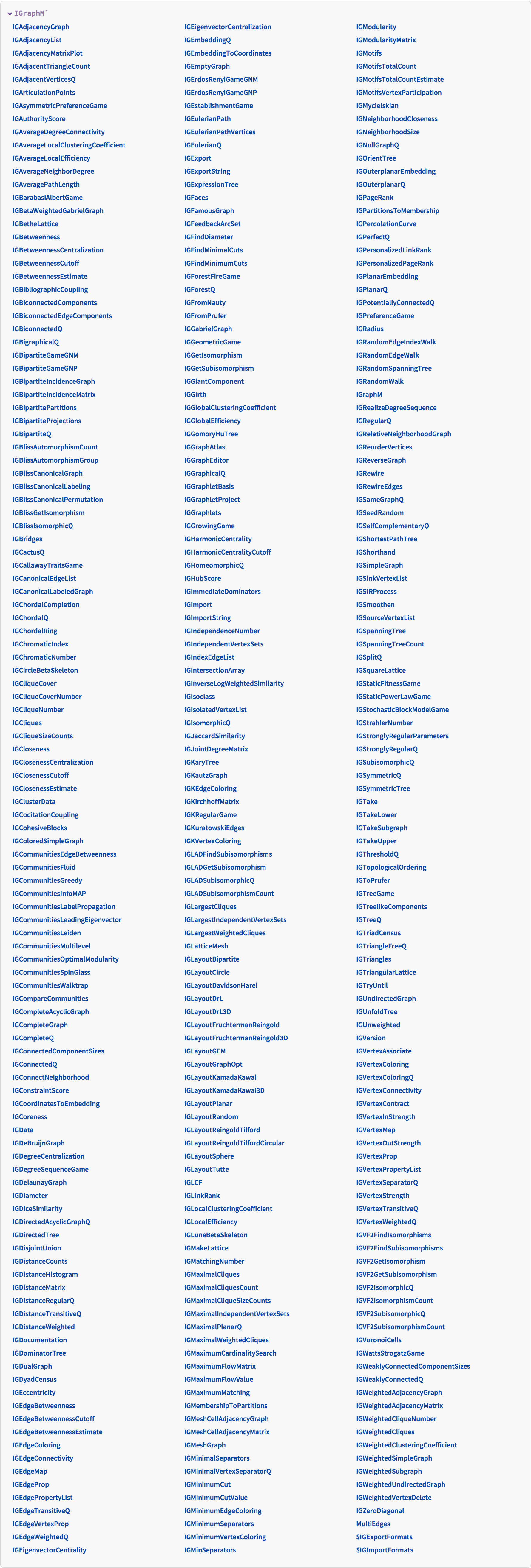
Or just type a question mark followed by the symbol’s name:
?IGVersion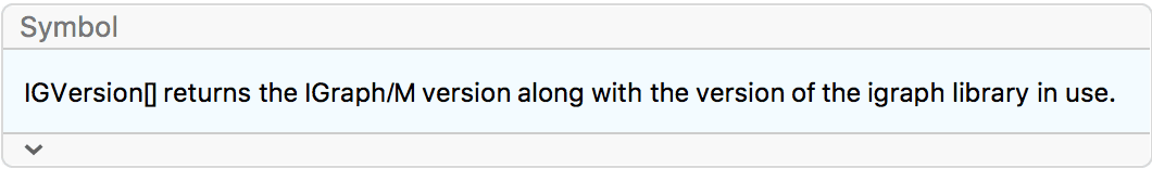
IGVersion[]"IGraph/M 0.6.5 (December 21, 2022) igraph 0.9.10-23-g5635203bd (Dec 21 2022) Mac OS X x86 (64-bit)"
IGraph/M functions work directly with Mathematica’s built-in
Graph datatype. No new special graph datatype is
introduced.
Let’s take a look at a few examples. Let us first generate a graph using the built-in functions of Mathematica.
SeedRandom[42];
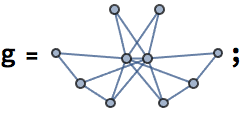
g = RandomGraph[BarabasiAlbertGraphDistribution[100, 2]]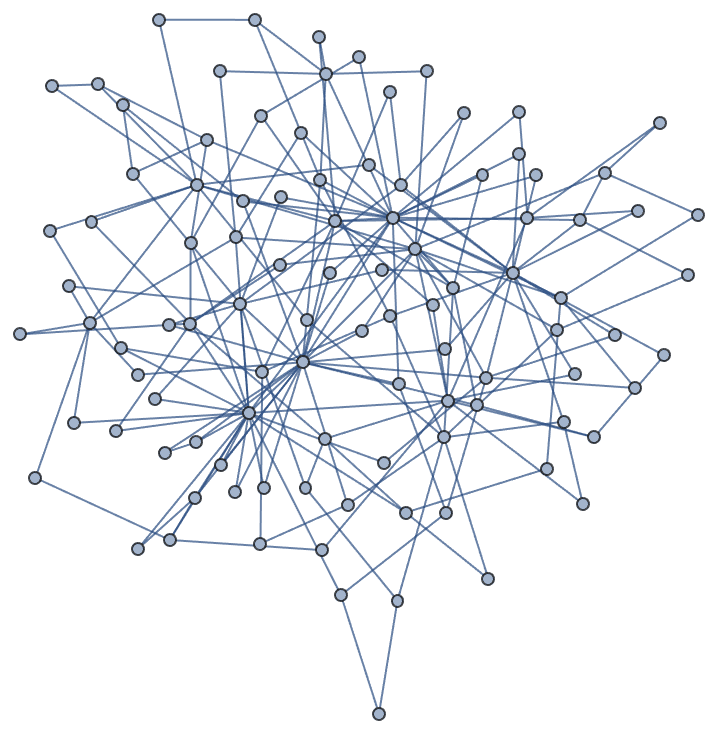
We can compute the betweenness centrality of each vertex either using IGraph/M, …
IGBetweenness[g]{1118.26, 1058.15, 540.601, 127.365, 1175.53, 678.175, 206.929, \ 128.576, 204.019, 535.316, 487.858, 391.669, 0., 135.039, 0., \ 52.5324, 104.28, 12.2286, 75.8798, 110.155, 68.8282, 13.9095, \ 46.4209, 99.3299, 0., 168.196, 213.871, 358.855, 0., 64.9572, \ 5.12619, 102.369, 17.978, 15.569, 95.7266, 8.45843, 25.4984, 13.0274, \ 0., 71.2012, 47.2895, 32.4444, 8.20833, 0., 27.0286, 10.9357, \ 4.60238, 0., 14.7095, 24.7944, 79.125, 7.38301, 22.0817, 43.9635, \ 11.7135, 10.9952, 40.8782, 11.2429, 0., 60.0431, 9.36667, 32.4529, \ 85.4487, 100.431, 15.205, 93.2876, 60.0548, 9.2, 0., 0., 10.512, \ 9.37438, 8.42222, 45.7937, 3.61667, 9.23333, 53.3897, 11.4012, \ 22.0959, 5.24091, 10.2647, 8.66017, 9.97438, 11.0429, 15.8765, \ 12.7798, 0., 30.1744, 0., 0., 4.0373, 9.7, 1., 10.4883, 0., 0., \ 13.7861, 13.8594, 1.7, 2.80952}
… or using Mathematica’s built-ins, and obtain the same result.
BetweennessCentrality[g]{1118.26, 1058.15, 540.601, 127.365, 1175.53, 678.175, 206.929, \ 128.576, 204.019, 535.316, 487.858, 391.669, 0., 135.039, 0., \ 52.5324, 104.28, 12.2286, 75.8798, 110.155, 68.8282, 13.9095, \ 46.4209, 99.3299, 0., 168.196, 213.871, 358.855, 0., 64.9572, \ 5.12619, 102.369, 17.978, 15.569, 95.7266, 8.45843, 25.4984, 13.0274, \ 0., 71.2012, 47.2895, 32.4444, 8.20833, 0., 27.0286, 10.9357, \ 4.60238, 0., 14.7095, 24.7944, 79.125, 7.38301, 22.0817, 43.9635, \ 11.7135, 10.9952, 40.8782, 11.2429, 0., 60.0431, 9.36667, 32.4529, \ 85.4487, 100.431, 15.205, 93.2876, 60.0548, 9.2, 0., 0., 10.512, \ 9.37438, 8.42222, 45.7937, 3.61667, 9.23333, 53.3897, 11.4012, \ 22.0959, 5.24091, 10.2647, 8.66017, 9.97438, 11.0429, 15.8765, \ 12.7798, 0., 30.1744, 0., 0., 4.0373, 9.7, 1., 10.4883, 0., 0., \ 13.7861, 13.8594, 1.7, 2.80952}
Let us now assign weights to the edges. Many IGraph/M functions,
including IGBetweenness, support edge weights.
wg = SetProperty[g, EdgeWeight -> RandomReal[1, EdgeCount[g]]];IGBetweenness[wg]{1569., 1509., 697., 506., 1510., 948., 173., 0., 106., 827., 663., \ 379., 0., 318., 0., 360., 0., 0., 83., 129., 1., 0., 227., 582., 0., \ 91., 236., 213., 0., 60., 0., 334., 1., 53., 549., 0., 0., 0., 0., \ 10., 0., 0., 0., 0., 68., 68., 17., 357., 27., 16., 80., 0., 0., 0., \ 437., 0., 0., 0., 52., 22., 0., 0., 62., 139., 93., 187., 1., 7., 0., \ 0., 0., 16., 0., 69., 10., 98., 0., 1., 4., 21., 0., 0., 0., 0., 0., \ 0., 0., 43., 0., 0., 98., 0., 0., 0., 0., 0., 0., 63., 25., 4.}
Notice that Mathematica 13.0 does not include functionality
to compute weighted vertex betweenness. The built-in function
BetweennessCentrality[] ignores the weights.
BetweennessCentrality[wg]{1118.26, 1058.15, 540.601, 127.365, 1175.53, 678.175, 206.929, \ 128.576, 204.019, 535.316, 487.858, 391.669, 0., 135.039, 0., \ 52.5324, 104.28, 12.2286, 75.8798, 110.155, 68.8282, 13.9095, \ 46.4209, 99.3299, 0., 168.196, 213.871, 358.855, 0., 64.9572, \ 5.12619, 102.369, 17.978, 15.569, 95.7266, 8.45843, 25.4984, 13.0274, \ 0., 71.2012, 47.2895, 32.4444, 8.20833, 0., 27.0286, 10.9357, \ 4.60238, 0., 14.7095, 24.7944, 79.125, 7.38301, 22.0817, 43.9635, \ 11.7135, 10.9952, 40.8782, 11.2429, 0., 60.0431, 9.36667, 32.4529, \ 85.4487, 100.431, 15.205, 93.2876, 60.0548, 9.2, 0., 0., 10.512, \ 9.37438, 8.42222, 45.7937, 3.61667, 9.23333, 53.3897, 11.4012, \ 22.0959, 5.24091, 10.2647, 8.66017, 9.97438, 11.0429, 15.8765, \ 12.7798, 0., 30.1744, 0., 0., 4.0373, 9.7, 1., 10.4883, 0., 0., \ 13.7861, 13.8594, 1.7, 2.80952}
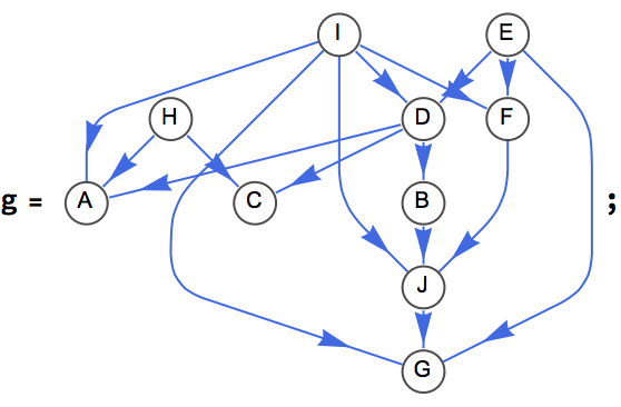
Let us delete the minimum feedback edge set to obtain an acyclic graph:
acg = EdgeDelete[g, IGFeedbackArcSet[g]]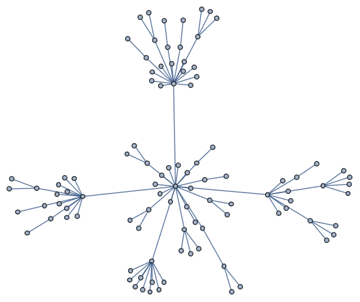
And try out a few of igraph’s layout algorithms.
{IGLayoutGraphOpt[acg], IGLayoutKamadaKawai[acg],
 IGLayoutFruchtermanReingold[acg]}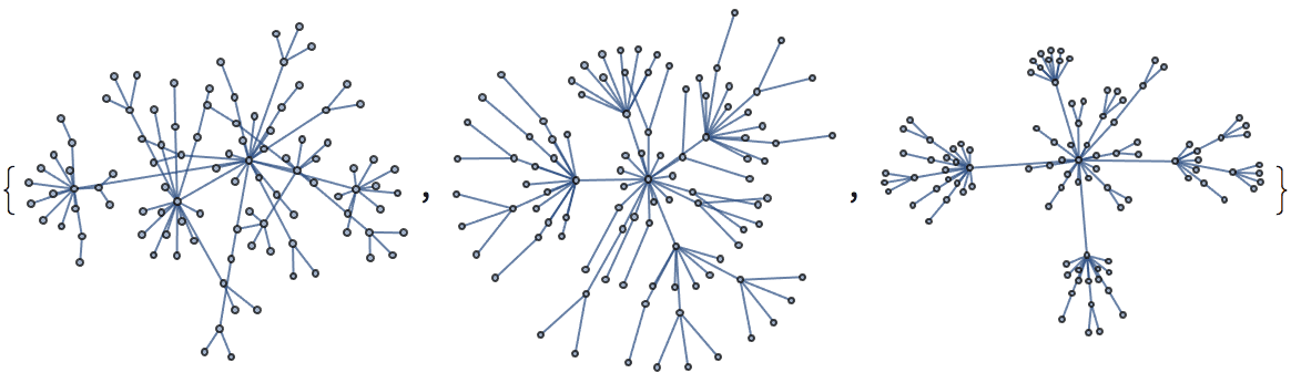
Layout functions typically have many options to tune:
Options[IGLayoutGraphOpt]{"MaxIterations" -> 500, "NodeCharge" -> 0.001, "NodeMass" -> 30, "SpringLength" -> 0, "SpringConstant" -> 1, "MaxStepMovement" -> 5, "Continue" -> False, "Align" -> True}
Increasing the number of iterations will usually improve the result.
IGLayoutGraphOpt[acg, "MaxIterations" -> 5000]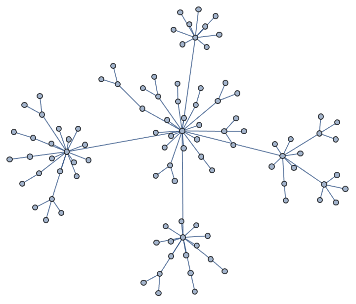
A final note
Please refer to the usage messages for information on how to use each function. For more information on the meaning of various function options, the algorithms used by the functions, references, etc. please refer to the C/igraph documentation. The igraph documentation provides article references for most nontrivial algorithms.
The following sections provide general information on each functionality area, and show common usage patterns.
All the graph creation functions in IGraph/M take any standard
Mathematica Graph option
such as VertexLabels, EdgeLabels,
VertexStyle, GraphStyle,
PlotTheme, etc.
IGLCF[{5, -5}, 7, GraphStyle -> "SmallNetwork"]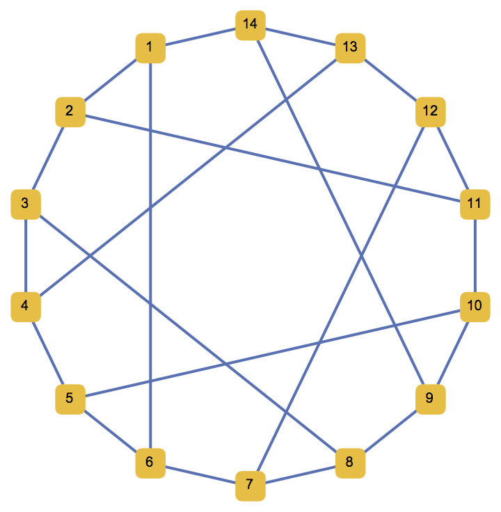
IGShorthand provides an easy way to create small graphs
from a simple and quick-to-type notation.
?IGShorthand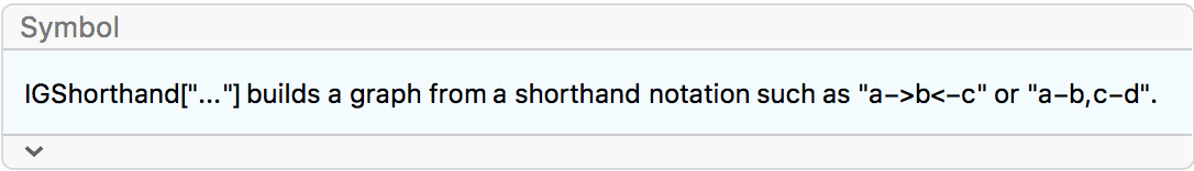
The available options are:
SelfLoops -> True keeps self-loops in the
graph.
MultiEdges -> True keeps parallel edges in the
graph.
Construct a cycle graph.
IGShorthand["1-2-3-4-1"]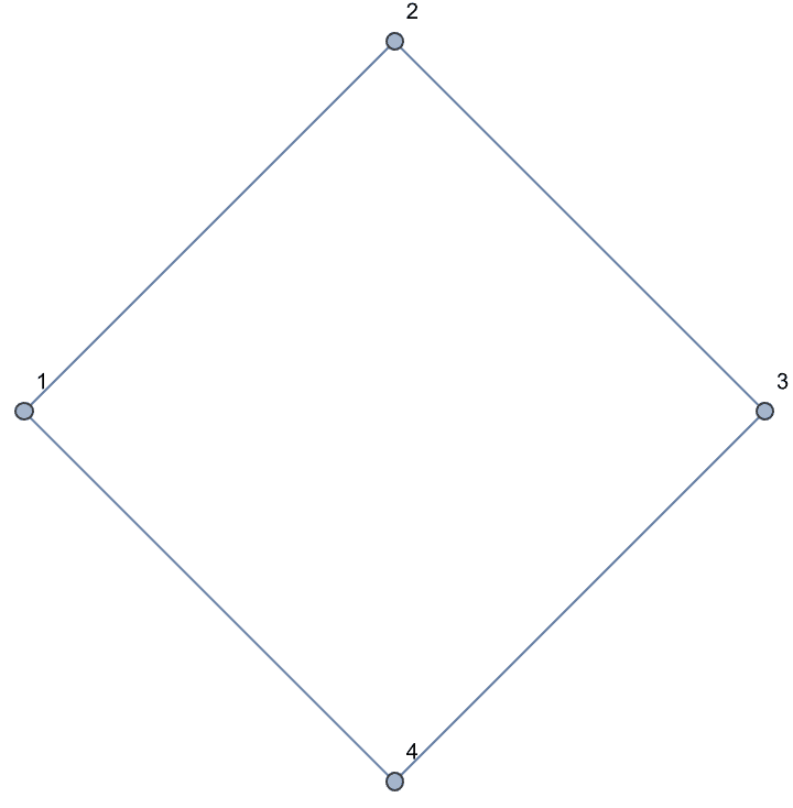
Vertex labels are shown by default. They can be turned off using
VertexLabels -> None.
IGShorthand["1-2-3-1", VertexLabels -> None]
The interpretation of - as directed or undirected is
controlled by the DirectedEdges option.
IGShorthand["1-2-3-1", DirectedEdges -> True]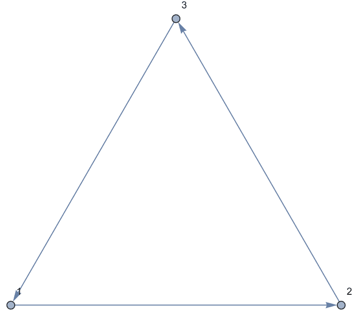
Directed edges can be input using ->,
<- or <->.
IGShorthand["Jim -> Suzy <- Joe"]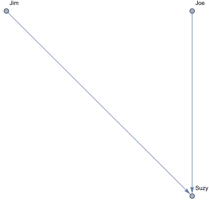
<-> is interpreted as a pair of directed
edges.
IGShorthand["1<->2->3"]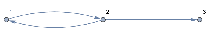
Mixed graphs, containing both directed and undirected edges, are supported. Note that mixed graphs are not allowed as input to most IGraph/M functions.
IGShorthand["1-2<-3"]![]()
Disconnected components are separated by commas.
IGShorthand["1, 2-3, 4-5-6"]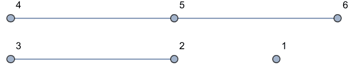
Groups of vertices can be given using the colon separator. Edges will be connected to each vertex in the group. This makes it easy to specify a complete graph …
IGShorthand["A:B:C:D:E -- A:B:C:D:E"]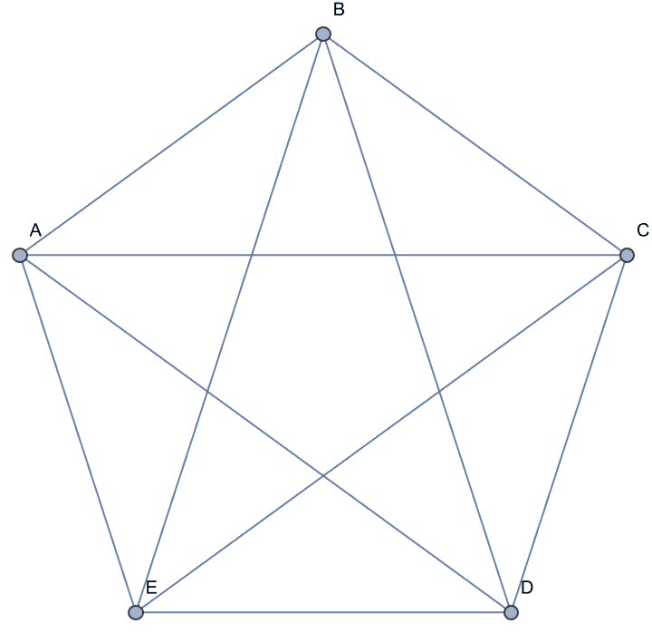
… or a complete bipartite graph.
IGLayoutBipartite@IGShorthand["a:b:c - 1:2:3:4"]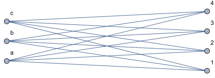
Vertex names are taken as strings, except when they can be interpreted as an integer.
IGShorthand["xyz - 137"] // VertexList // InputForm{"xyz", 137}Spaces are allowed in vertex names, and edges can be specified using
any number of - characters.
IGShorthand["Sophus Lie --- Camille Jordan"]![]()
Self-loops and parallel edges are removed by default because these
are often created as an undesired by-product of vertex groups. They can
be re-enabled using the SelfLoops or
MultiEdges options when desired.
IGShorthand["1:2:3 - 1:2:3", SelfLoops -> True]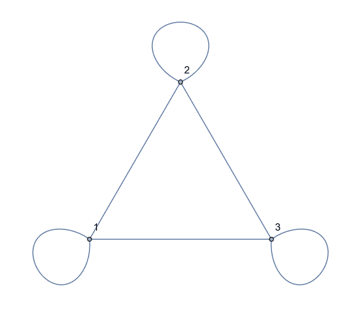
IGShorthand["1:2:3 - 1:2:3", SelfLoops -> True, MultiEdges -> True]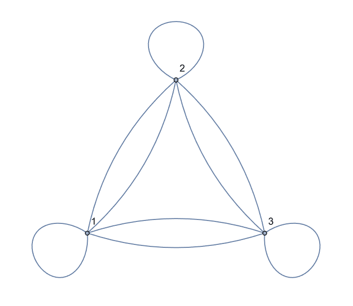
IGShorthand["1-2-1-3", MultiEdges -> True]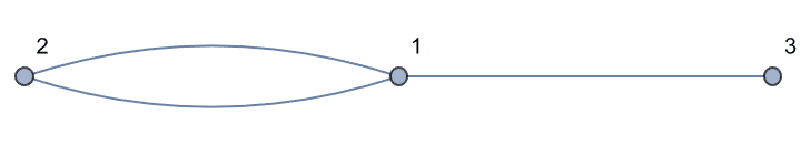
The vertex order will follow the order of appearance of vertices in the input string. To control the order, simply list vertices at the beginning of the shorthand specification.
IGShorthand["4-3-1-2-4"] // VertexList{4, 3, 1, 2}
IGShorthand["1,2,3,4, 4-3-1-2-4"] // VertexList{1, 2, 3, 4}
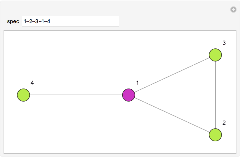
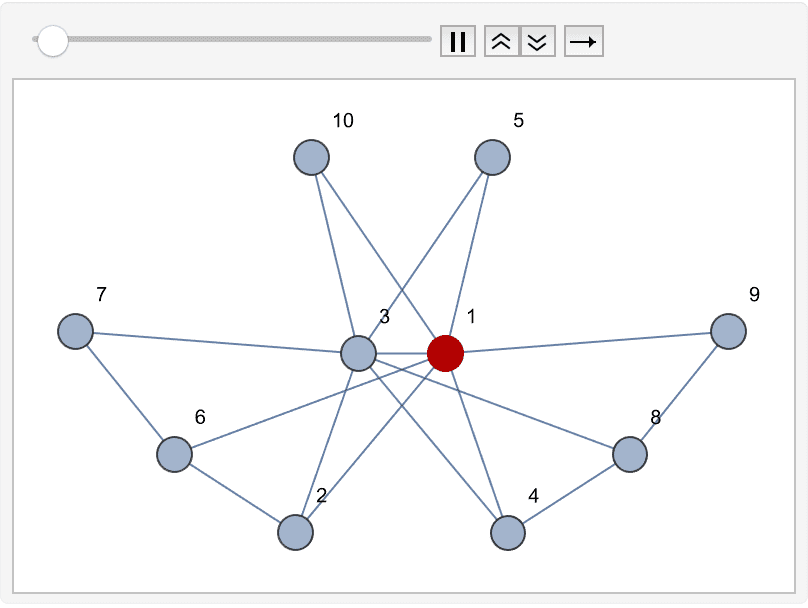
Create an interactive graph editor that dynamically visualizes betweenness.
Manipulate[
 IGShorthand[spec, VertexSize -> {"Scaled", 0.06},
   EdgeStyle -> Gray] //
  IGVertexMap[ColorData["NeonColors"],
   VertexStyle -> IGBetweenness/*Rescale],
 {{spec, "1-2-3-1-4"},
  InputField[#, String, ContinuousAction -> True] &},
 Initialization :> Needs["IGraphM`"]
 ]
?IGEmptyGraph
IGEmptyGraph is a convenience function for creating
graphs with no edges.
Create a null graph.
IGEmptyGraph[] // VertexCount0
Create an empty graph on 15 vertices.
IGEmptyGraph[15]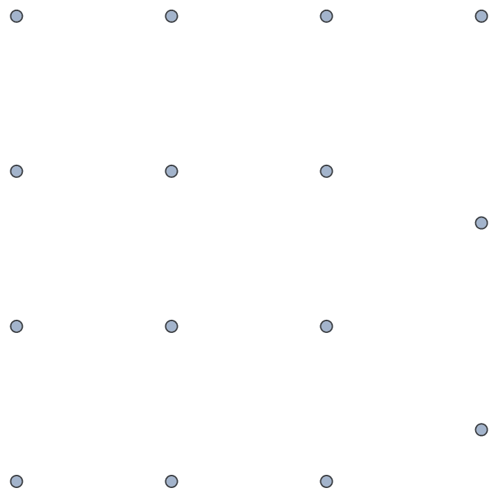
The built-in EmptyGraphQ returns True for
these graphs.
EmptyGraphQ[%]True
?IGLCF
![]() creates a graph based on the LCF
notation
creates a graph based on the LCF
notation![]() .
.
The Möbius–Kantor graph is [5, -5]^8.
IGLCF[{5, -5}, 8, GraphStyle -> "DiagramGreen"]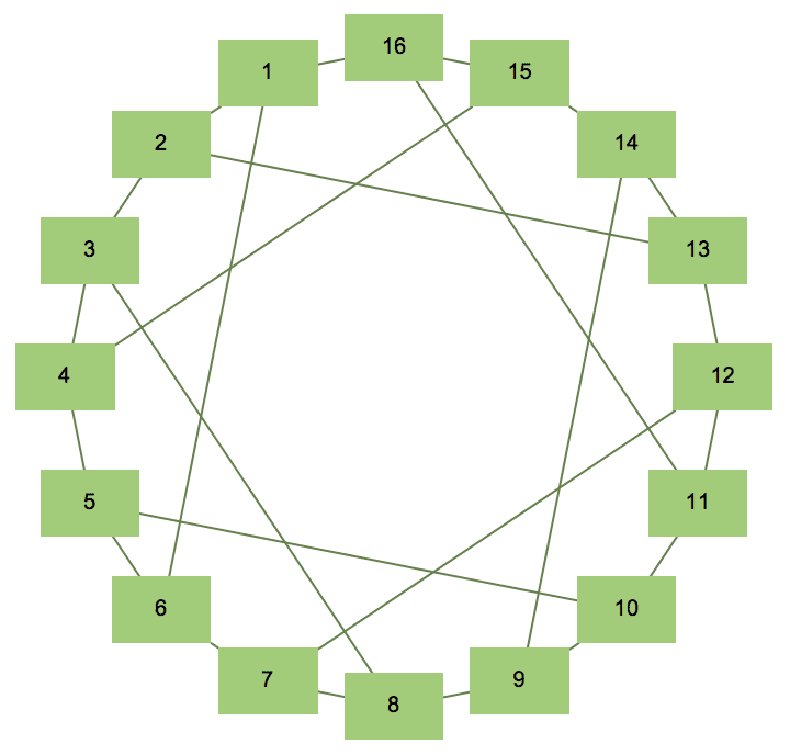
The Pappus graph is [5, 7, -7, 7, -7, -5]^3.
IGLCF[{5, 7, -7, 7, -7, -5}, 3, GraphStyle -> "ThickEdge"]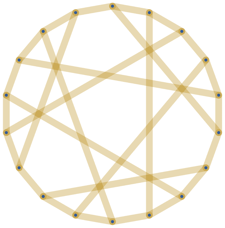
The cuboctahedral graph is [4, 2]^6.
IGLayoutKamadaKawai3D@IGLCF[{4, 2}, 6]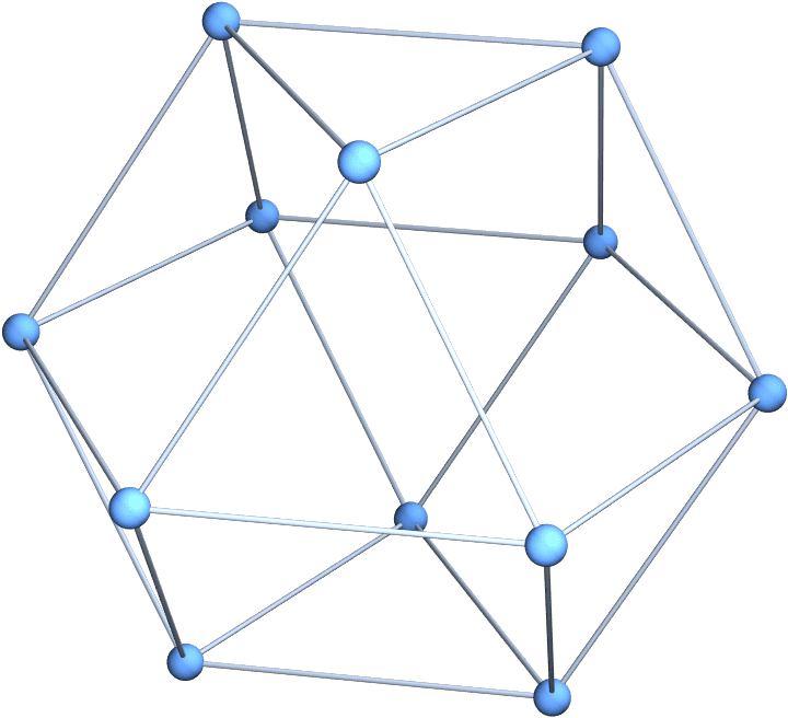
?IGChordalRing
IGChordalRing[n, w] constructs an extended chordal ring
based on the offset specification vector or matrix \(w\) as follows:
It creates a cycle graph (i.e. ring) on \(n\) vertices.
For each vertex \(i\) on the ring, it adds a chord to a vertex \(w[[(i \bmod p)]]\) steps ahead counter-clockwise on the ring.
If \(w\) is a matrix, the procedure is carried out for each row.
The number of vertices \(n\) must be an integer multiple of the number of columns in the matrix \(w\).
The available options are:
DirectedEdges -> True creates a graph with
directed edges.
SelfLoops -> False prevents the creation of
self-loops.
MultiEgdes -> False prevents the creation of
multi-edges.
Create an extended chordal graph.
IGChordalRing[15, {3, 4, 8}, GraphStyle -> "Business"]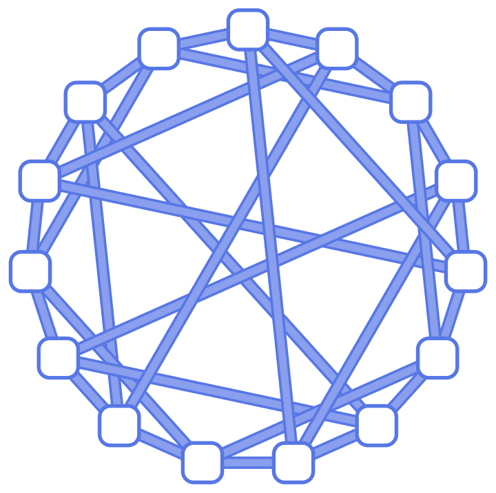
Negative offsets are allowed.
IGChordalRing[15, {{3, 4, 8}, {-3, -4, -8}}]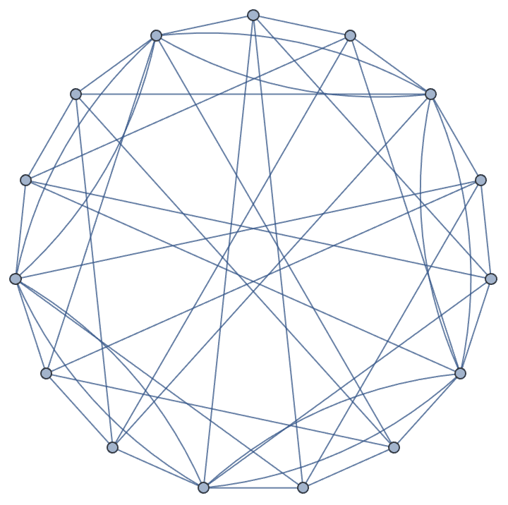
IGChordalGraph may create self-loops or multi-edges.
This can be prevented by setting the SelfLoops or
MultiEdges options to False.
IGChordalRing[15, {{3, 4, 8}, {-3, -4, -8}}, MultiEdges -> False]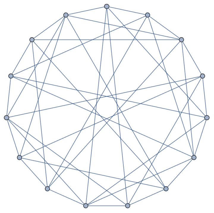
Create a chordal graph with directed edges.
IGChordalRing[8, {2, 3}, DirectedEdges -> True,
 GraphStyle -> "DiagramGold"]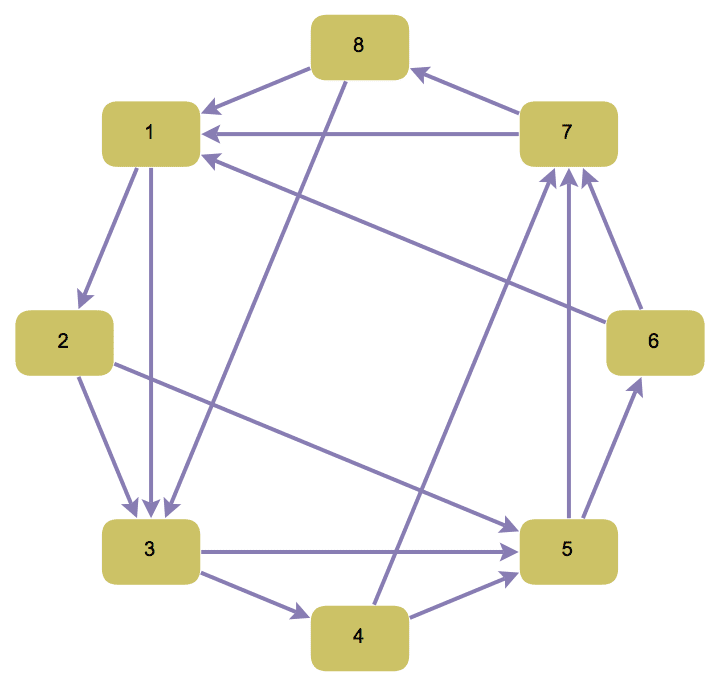
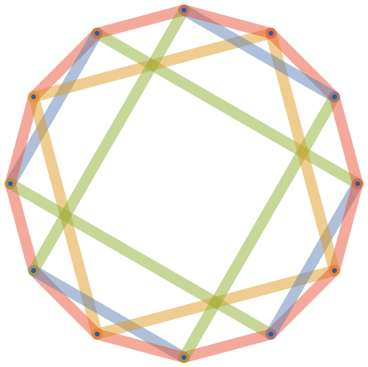
Colour the chords of the ring based on which entry of the \(w\) vector they correspond to.
w = {2, 3, 4};
IGChordalRing[12, w, GraphStyle -> "ThickEdge",
  EdgeStyle -> Opacity[1/2]] // IGEdgeMap[
  ColorData[97],
  EdgeStyle -> Function[g,
    Table[
     If[i <= VertexCount[g], 0, Mod[i, Length[w], 1]], {i,
      EdgeCount[g]}]
    ]
  ]
?IGSquareLattice
![]() creates a square lattice graph of the given dimensions. The available
options are:
creates a square lattice graph of the given dimensions. The available
options are:
"Radius" controls the size of the neighbourhood
within which vertices will be connected.
"Periodic" -> True creates a periodic
lattice.
"Mutual" -> True inserts directed edges in both
directions when DirectedEdges -> True is used.
In previous versions, IGSquareLattice was called
IGMakeLattice. This name can still be used as a synonym for
the sake of backwards compatibility, however, it will be removed in a
future version.
To create other types of lattices, see IGTriangleLattice
and IGLatticeMesh.
IGSquareLattice[{3, 4}, GraphStyle -> "VintageDiagram"]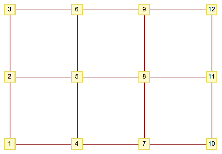
IGSquareLattice[{10, 10}, "Periodic" -> True]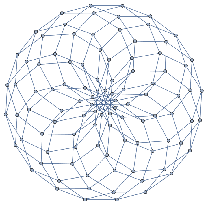
Graph3D@IGSquareLattice[{5, 4, 3}, GraphStyle -> "Prototype"]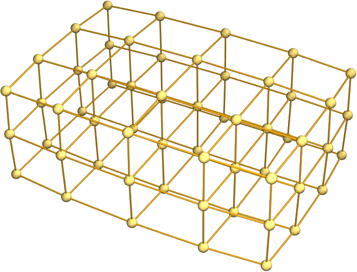
Graph3D@IGSquareLattice[{2, 5}, DirectedEdges -> True,
  "Periodic" -> True, PlotTheme -> "NeonColor"]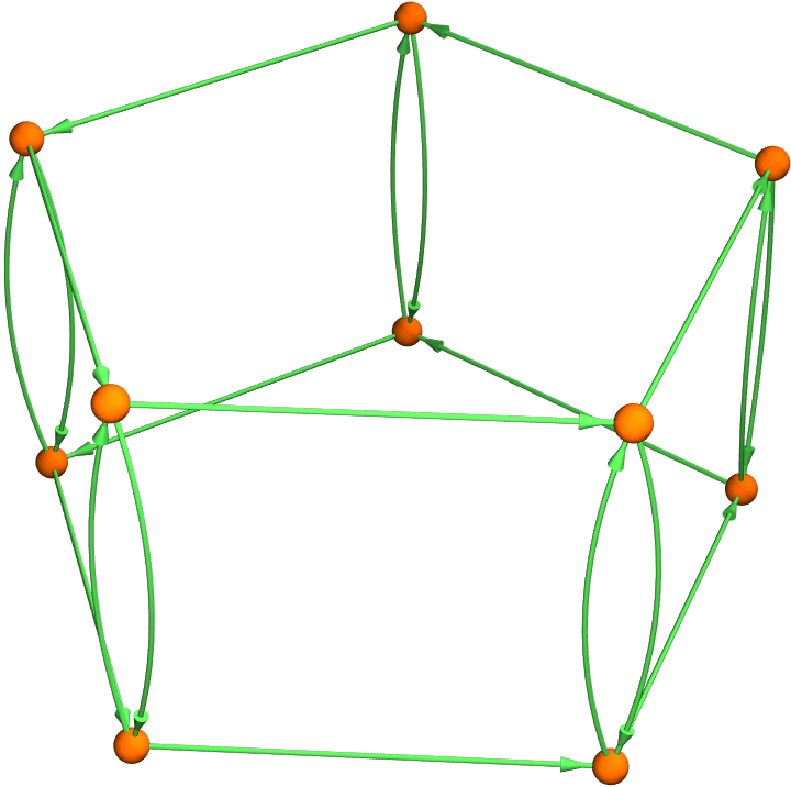
?IGTriangularLattice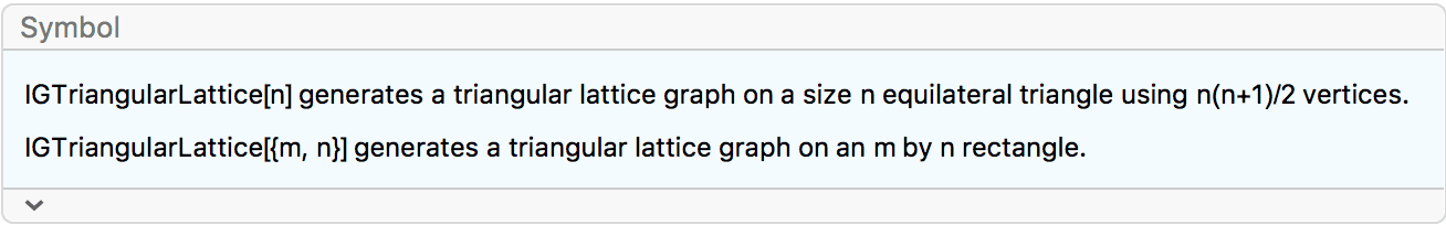
IGTriangularLattice can create a triangular grid graph
in the shape of a triangle or a rectangle. To generate other types of
lattices, see IGSquareLattice and
IGLatticeMesh.
The available options are:
DirectedEdges -> True creates a directed
graph.
"Periodic" -> True creates a periodic
lattice.
Generate a triangular lattice on an equilateral triangle with 6 vertices along each of its edges.
IGTriangularLattice[6, GraphStyle -> "SmallNetwork"]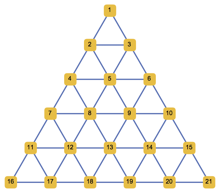
Create a directed triangle lattice on a rectangle. Notice the vertex labelling and that the arrows are oriented from smaller index vertices to larger index ones, making this an acyclic graph.
IGTriangularLattice[{4, 4}, DirectedEdges -> True,
 VertexShapeFunction -> "Name", PerformanceGoal -> "Quality"]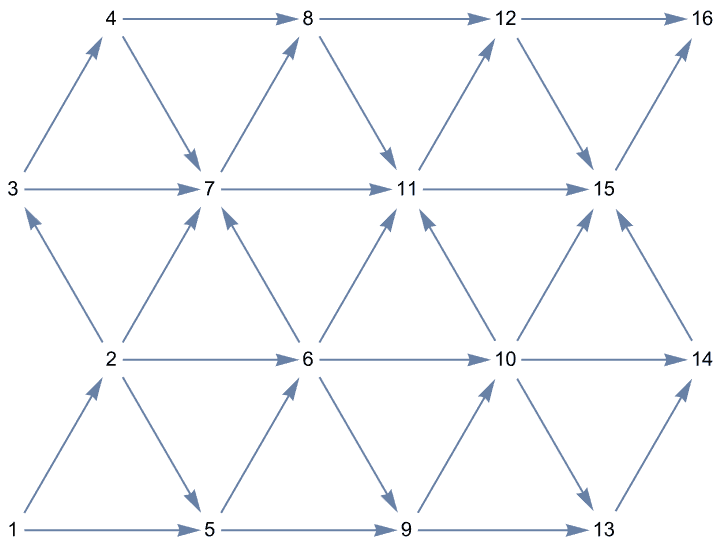
Create a triangle lattice and colour its vertices.
IGTriangularLattice[{8, 6}, VertexSize -> Large, EdgeStyle -> Gray] //
  IGVertexMap[ColorData[98], VertexStyle -> IGMinimumVertexColoring]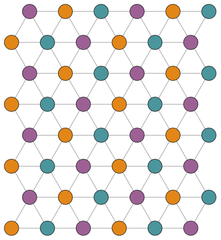
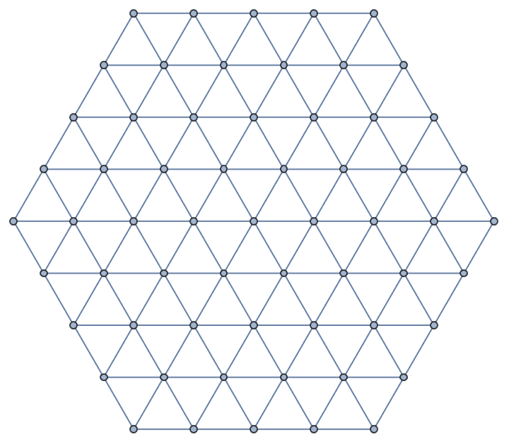
Take a hexagonal subgraph of a triangle lattice.
g = IGTriangularLattice[13];
center = First@GraphCenter[g];
VertexDelete[g,
 Complement[VertexList[g], AdjacencyList[g, center, 4], {center}]
 ]
Create a periodic (i.e. toroidal topology) triangle lattice.
Graph3D@IGTriangularLattice[{24, 8}, "Periodic" -> True]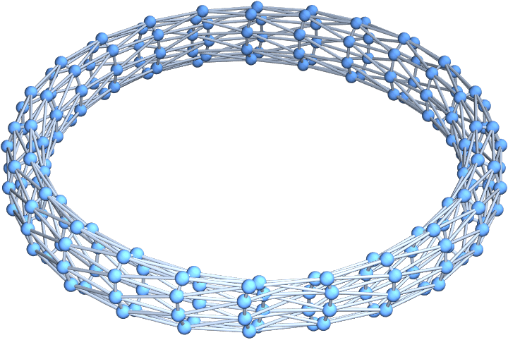
?IGKaryTree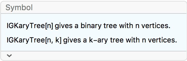
The available options are:
DirectedEdges -> True creates a directed tree.IGKaryTree[15]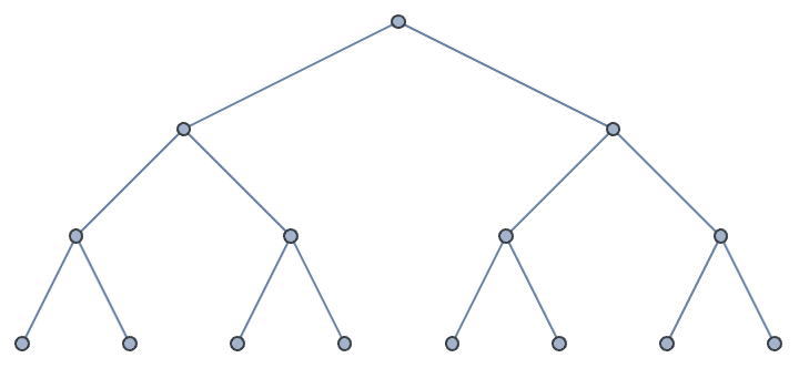
IGKaryTree[10, 3, DirectedEdges -> True]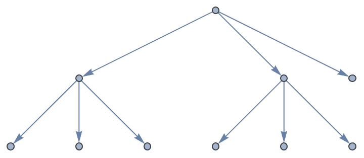
?IGSymmetricTree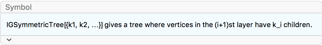
IGSymmetricTree creates a tree where successive layers
(i.e. vertices at the same distance from the root) have the specified
number of children.
Create a tree where the root has 4 children, its children have 3 children, and so on.
IGSymmetricTree[{4, 3, 2, 1}]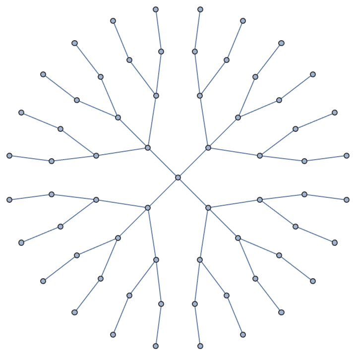
Create a directed tree.
IGSymmetricTree[{4, 2}, DirectedEdges -> True]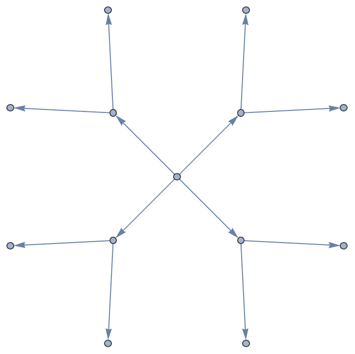
IGSymmetricTree is guaranteed to label vertices in
breadth-first order. Deeper layers have higher integer labels.
IGSymmetricTree[{3, 3}, GraphStyle -> "DiagramBlue"]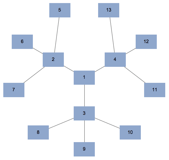
?IGBetheLattice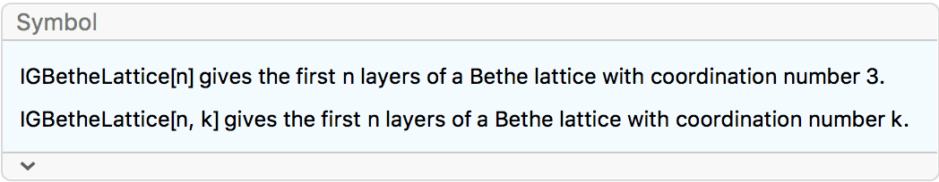
A Bethe lattice, also called a regular tree, is an infinite tree in
which all vertices have the same degree.
IGBetheLattice[n, k] computes the first n
layers of such a tree. Each non-leaf vertex will have degree
k. The default degree is 3.
IGBetheLattice differs from
CompleteKaryTree in that the degree of the root will be the
same as the degree of other non-lead nodes.
IGBetheLattice[5, GraphStyle -> "Prototype", VertexSize -> Large]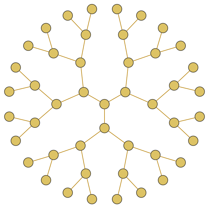
Generate a tree where non-leaf nodes have total degree 5, and use directed edges.
IGBetheLattice[5, 4, DirectedEdges -> True]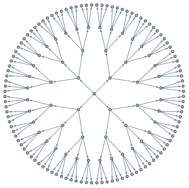
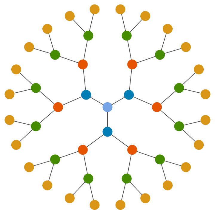
Colour vertices based on their distance from the root (i.e. the “layer” they are part of).
IGVertexMap[
 ColorData[68],
 VertexStyle -> (First@IGDistanceMatrix[#, {1}] &),
 IGBetheLattice[5, GraphStyle -> "BasicBlack", VertexSize -> 0.4]
 ]
Visualize the nested line graph of a degree-4 regular tree.
Graph3D@Nest[LineGraph, IGBetheLattice[5, 4], 2]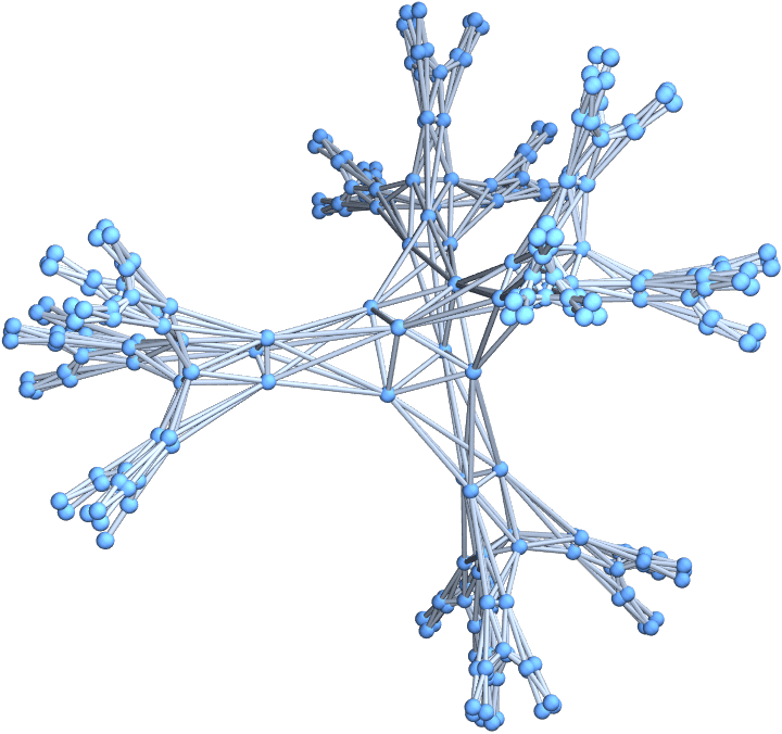
?IGFromPrufer
A Prüfer sequence is a unique representation of an \(n\)-vertex labelled tree as \(n-2\) integers between \(1\) and \(n\).
IGFromPrufer[{1, 1, 2, 2}, VertexLabels -> "Name"]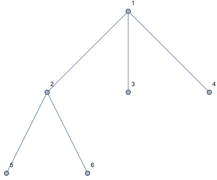
Use IGToPrufer to convert a tree back to its Prüfer
sequence.
IGToPrufer[%]{1, 1, 2, 2}
Generate all labelled trees on 4 nodes:
IGFromPrufer[#, VertexLabels -> "Name"] & /@ Tuples[Range[4], {2}]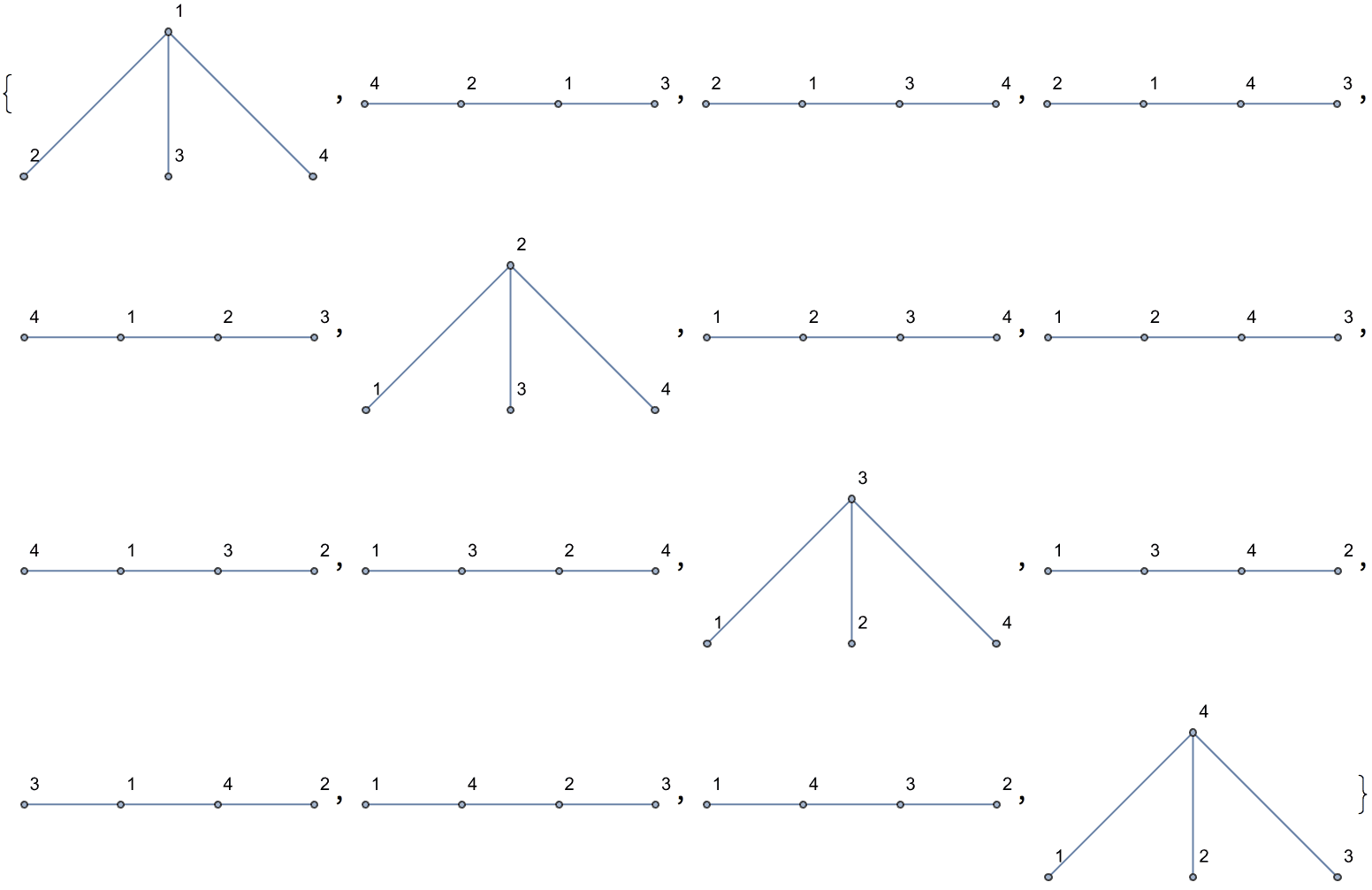
Of these, only two are non-isomorphic.
DeleteDuplicates[CanonicalGraph /@ %]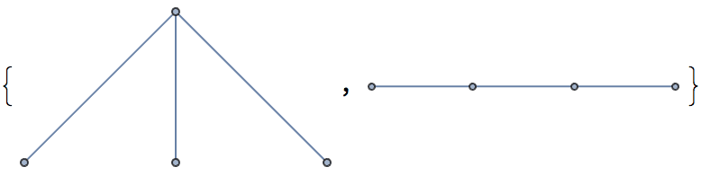
?IGExpressionTree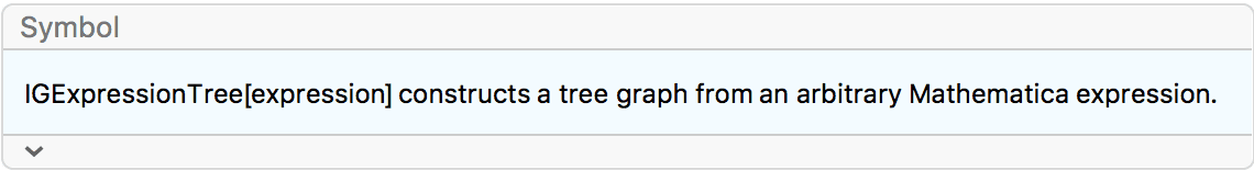
IGExpressionTree constructs the tree graph corresponding
to an arbitrary Mathematica expression. The vertices of the
tree will be the positions of the corresponding subexpressions.
IGExpressionTree takes all standard Graph
options. The VertexLabels option takes the following
special values:
VertexLabels -> "Head" labels branch vertices
with the Head of the corresponding subexpression and leaf
vertices with the corresponding atomic expression.
VertexLabels -> "Subexpression" labels vertices
with the corresponding subexpression.
VertexLabels -> "Name" labels vertices with their
name, i.e. the position of the corresponding subexpression.
VertexLabels -> None uses no labels.
IGExpressionTree constructs a graph corresponding to the
structure of a Mathematica expression.
tree = IGExpressionTree[expr = 1 + x^2]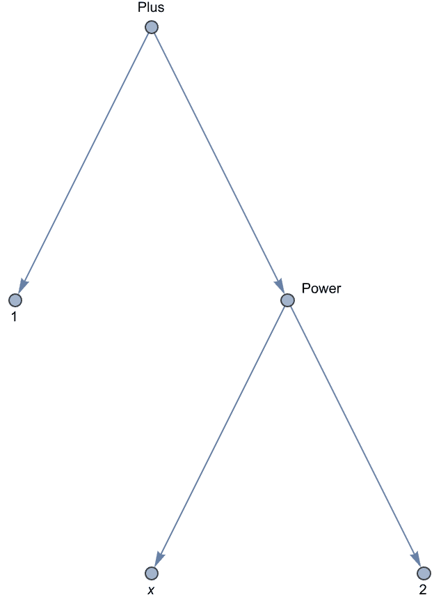
The expression tree is similar to what TreeForm
displays, but unlike TreeForm’s output, it is a
Graph object that works with all graph functions.
TreeForm[expr]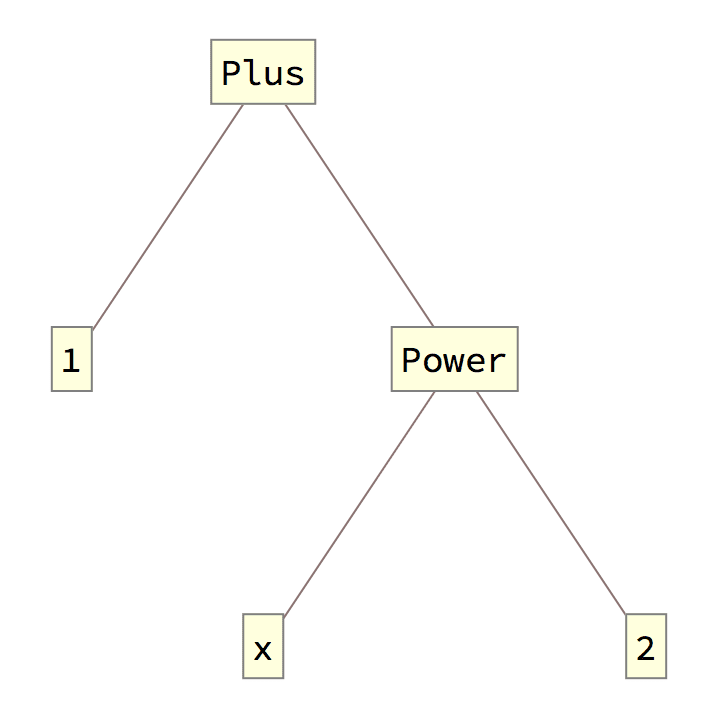
The vertex names are the position specifications of the corresponding subexpressions.
VertexList[tree]{{1}, {2, 1}, {2, 2}, {2}, {}}
Extract[expr, %]{1, x, 2, x^2, 1 + x^2}
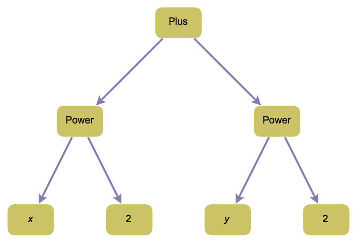
Place the vertex labels in the centre and construct an undirected graph.
IGExpressionTree[x^2 + y^2,
 GraphStyle -> "DiagramGold",
 VertexLabels -> Placed["Head", Center], VertexSize -> Large
 ]
Create an undirected graph, labelled with subexpressions.
IGExpressionTree[Normal[Sin[x] + O[x]^5], DirectedEdges -> False,
 VertexLabels -> "Subexpression"]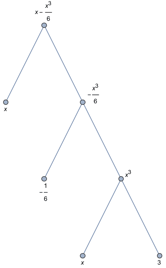
Certain trees are easier to construct through their corresponding nested expression.
IGExpressionTree[#, VertexLabels -> "Index"] & /@ Groupings[5, 3]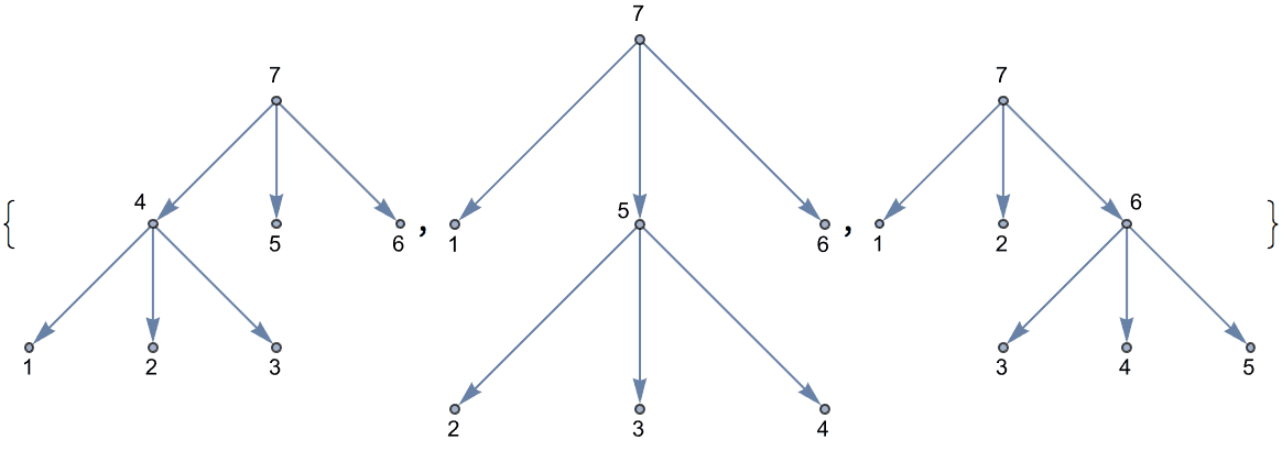
An equivalent of IGSymmetricTree can be easily
implemented using IGExpressionTree.
IGExpressionTree[ConstantArray[1, {3, 4, 5}], VertexLabels -> None,
 GraphLayout -> "RadialEmbedding"]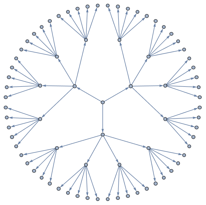
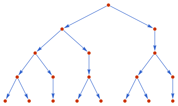
Define a tree through a substitution system.
IGExpressionTree[
 Nest[ReplaceAll[{0 -> {0, 1}, 1 -> {0}}], {0, 1}, 3],
 VertexLabels -> None, GraphStyle -> "VibrantColor"
 ]
To format each node so that it fits a label, it is necessary to set
an explicit VertexShapeFunction.
IGExpressionTree[First@Roots[x^2 + a x + 1 == 0, x],
   VertexLabels -> "Subexpression",
   PerformanceGoal -> "Quality",
   ImageSize -> 280
   ] //
  IGVertexMap[
   Function[e, Inset[Panel[e], #1] &],
   VertexShapeFunction -> IGVertexProp[VertexLabels]
   ] // RemoveProperty[#, VertexLabels] &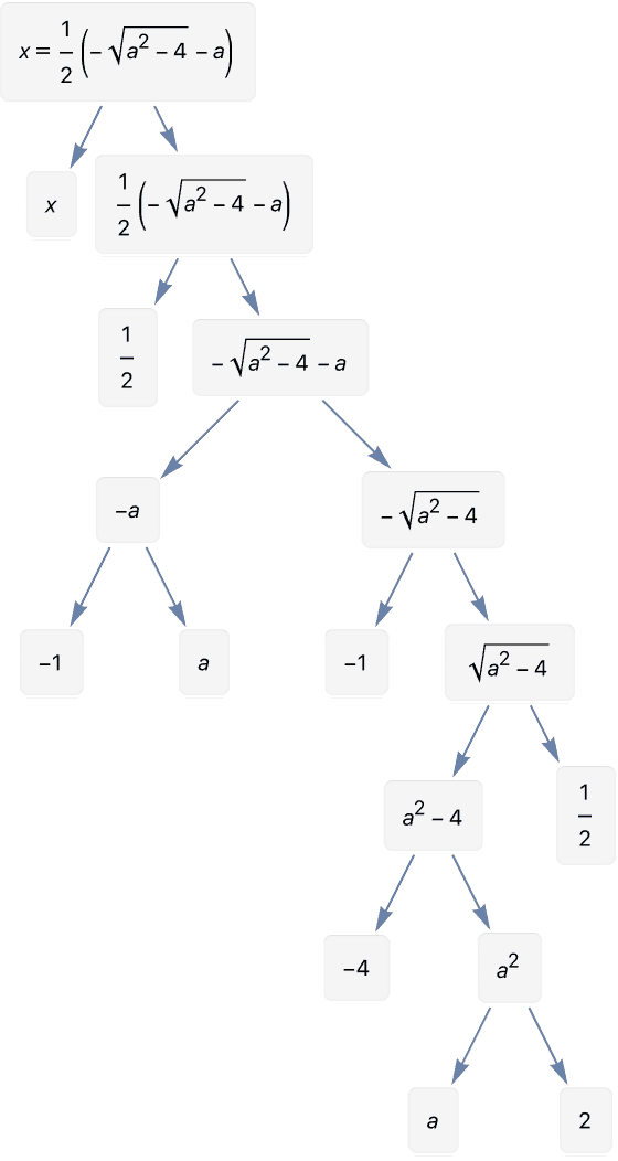
?IGCompleteGraph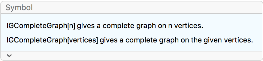
The available options are:
DirectedEdges -> True creates a directed
graph.
SelfLoops -> True includes self-loops.
Create an undirected complete graph with loops.
IGCompleteGraph[5, SelfLoops -> True]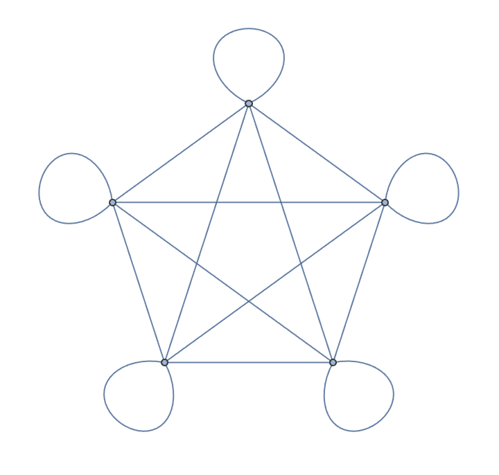
Create a directed complete graph with loops.
IGCompleteGraph[6, SelfLoops -> True, DirectedEdges -> True]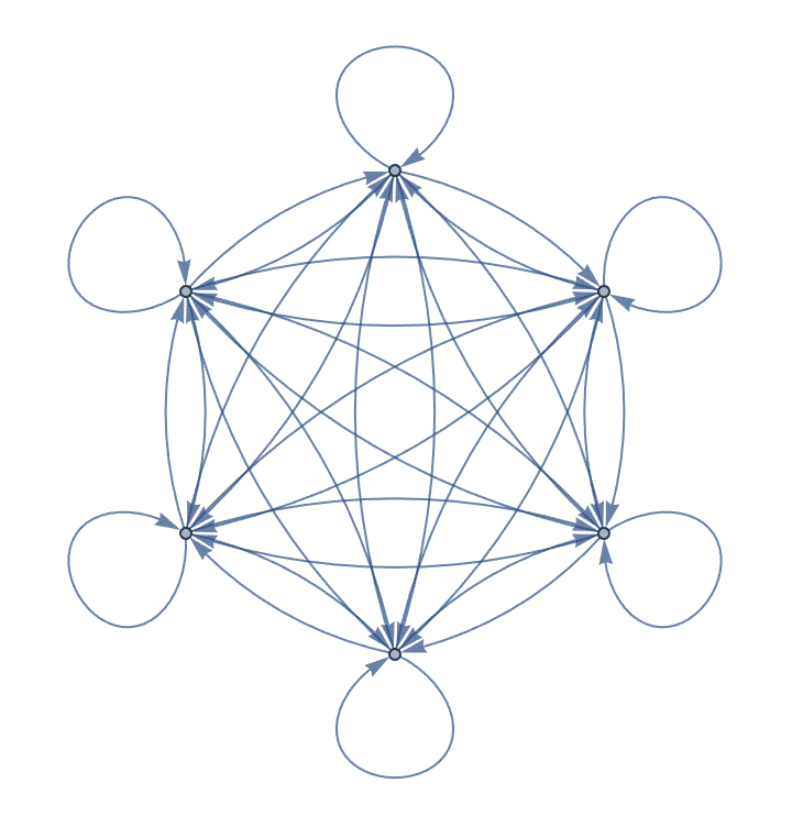
Create a list of complete graphs starting with the null graph.
IGCompleteGraph /@ Range[0, 3]
Create a complete graph on the given vertices.
IGCompleteGraph[{"a", "b", "c", "d"}, GraphStyle -> "DiagramBlue"]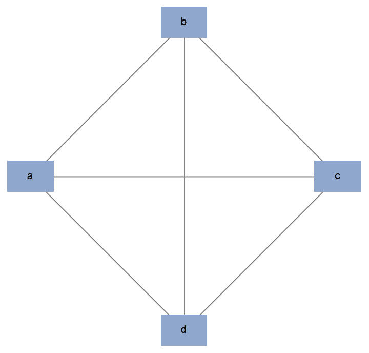
?IGCompleteAcyclicGraph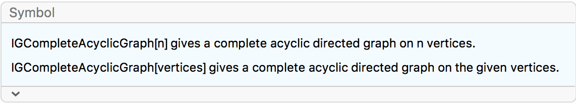
Create a complete acyclic directed graph on 5 vertices.
IGCompleteAcyclicGraph[5]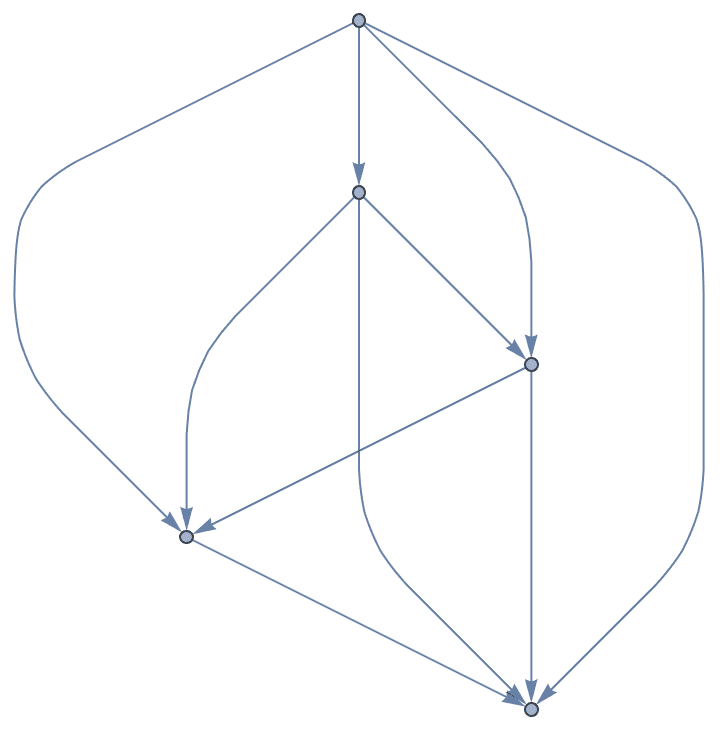
Create a complete acyclic graph on the given vertices. The directed edges always run from vertices that appear earlier in the list to those that appear later.
IGCompleteAcyclicGraph[CharacterRange["a", "f"],
 GraphStyle -> "DiagramGold"]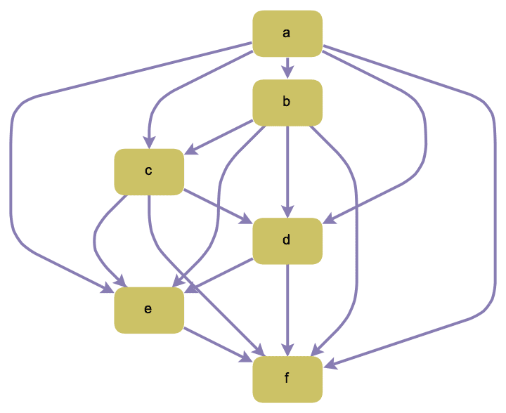
?IGKautzGraph
The vertices of the Kautz graph \(K_m^n\) are strings of length \(n+1\), composed of \(m+1\) distinct symbols, with the restriction that two adjacent symbols in the string may not be the same. A vertex \(s_1s_2\text{$\ldots $s}_ns_{n+1}\) connects to all other vertices of the form \(s_2\text{$\ldots $s}_{n+1}x\), where \(x\) can be any symbol distinct from \(s_{n+1}\).
The Kautz graph \(K_m^n\) has \((m+1) m^n\) vertices, with each vertex having in-degree and out-degree \(m\). Therefore, it has \((m+1) m^{n+1}\) edges.
VertexCount@IGKautzGraph[3, 2] == (3 + 1)*3^2True
VertexOutDegree@IGKautzGraph[3, 2]{3, 3, 3, 3, 3, 3, 3, 3, 3, 3, 3, 3, 3, 3, 3, 3, 3, 3, 3, 3, 3, 3, 3, \ 3, 3, 3, 3, 3, 3, 3, 3, 3, 3, 3, 3, 3}
The line graph of Kautz graph \(K_m^n\) is \(K_m^{n+1}\).
IGIsomorphicQ[
 LineGraph@IGKautzGraph[2, 2],
 IGKautzGraph[2, 3]
 ]
True
Visualize the Kautz graph \(K_2^3\) on 3 characters with string length 4 in three dimensions.
Graph3D@IGKautzGraph[2, 3]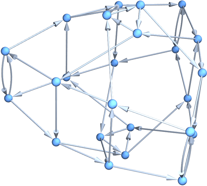
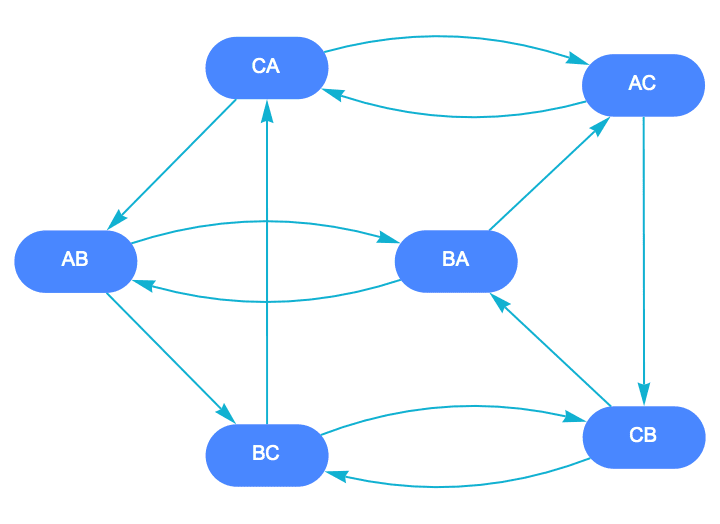
Label the vertices of the Kautz graph on 3 characters with string length 2.
labels =
  StringJoin /@ DeleteCases[Tuples[{"A", "B", "C"}, {2}], {c_, c_}];
IGKautzGraph[2, 1,
 VertexLabels -> Thread[Range[6] -> (Placed[#, Center] &) /@ labels],
 VertexSize -> Large, VertexShapeFunction -> "Capsule",
 PerformanceGoal -> "Quality",
 PlotTheme -> "CoolColor", VertexLabelStyle -> White
 ]
?IGDeBruijnGraph
IGDeBruijnGraph[3, 2, GraphStyle -> "BackgroundBlue",
 EdgeStyle -> Thick]
?IGRealizeDegreeSequence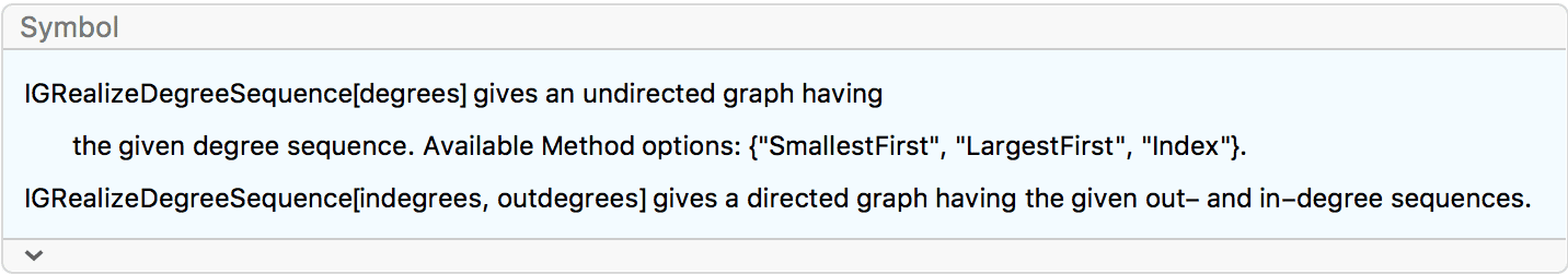
This function constructs an undirected graph with the given degree
sequence, or a directed graph with the given in- and out-degree
sequences. For constructing simple graphs, it uses the Havel–Hakimi
algorithm (undirected case) or Kleitman–Wang algorithm (directed case).
These algorithms work by selecting a “hub” vertex, and connecting up all
its free (out-)degrees to other vertices with the largest degrees. In
the directed case, the “largest” degrees are determined by lexicographic
ordering of (in, out)-degree pairs. For constructing a loop-free
multigraph, a similar algorithm is used, but the hub is connected to
only one other vertex in each step, instead of to as many as its degree.
If self-loops are allowed as well, the same algorithm is used, and if a
loop-free result cannot be created, an appropriate number of self-loops
will be added to the very last hub. The order in which hub vertices are
selected is controlled by the Method option.
To randomly sample multiple realizations of a degree sequence, use
IGDegreeSequenceGame, or first create a single graph with
IGRealizeDegreeSequence, then randomly rewire it using
IGRewire.
The available options are:
SelfLoops -> True allows creating self-loops
(disallowed by default).
MultiEdges -> True allows creating multi-edges
(disallowed by default).
The Method option controls the order in which hub
vertices are chosen.
Available Method option values:
"SmallestFirst" will choose a smallest-degree vertex
in each step of the algorithm (this is the default). This results in a
disassortative network. In the undirected case, this method is
guaranteed to construct a connected graph, if one exists, both when
constructing simple graphs or multigraphs. See Horvát and Modes (2020), as
well as http://szhorvat.net/pelican/hh-connected-graphs.html
for the proof. In the directed case, it tends to construct
weakly-connected graphs, but this is not guaranteed.
"LargestFirst" will choose a largest-degree vertex.
This results in an assortative network. This method tends to construct
disconnected graphs. This is the most common variant of the Havel–Hakimi
algorithm implemented in other packages.
"Index" will choose vertices in the order of their
indices.
degseq = VertexDegree@IGGiantComponent@RandomGraph[{50, 50}]{3, 4, 4, 4, 2, 1, 2, 3, 3, 1, 2, 3, 2, 3, 1, 5, 2, 4, 3, 1, 2, 5, 4, \ 3, 1, 3, 2, 1, 2, 2, 3, 1, 3, 1, 1, 1, 1, 1}
The default Method -> "SmallestFirst" tends to create
highly disassortative graphs. The result is guaranteed to be connected
if the input degree sequence was potentially connected.
IGRealizeDegreeSequence[degseq]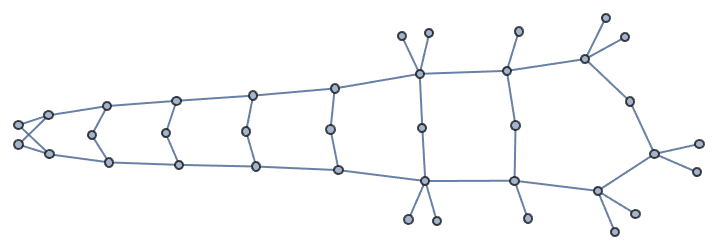
N@GraphAssortativity[%]-0.524347
Method -> "LargestFirst" tends to create highly
assortative disconnected graphs.
IGRealizeDegreeSequence[degseq, Method -> "LargestFirst"]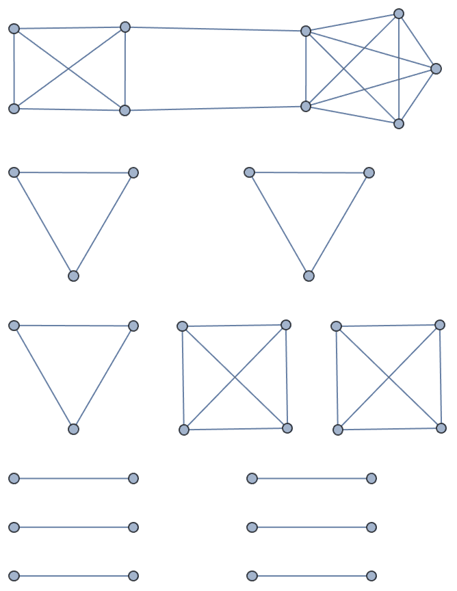
N@GraphAssortativity[%]0.904728
Allow parallel edges.
IGRealizeDegreeSequence[degseq, MultiEdges -> True,
   Method -> #] & /@ {"SmallestFirst", "LargestFirst", "Index"}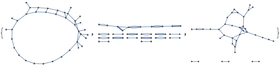
Create a directed graph.
g = IGBarabasiAlbertGame[50, 1]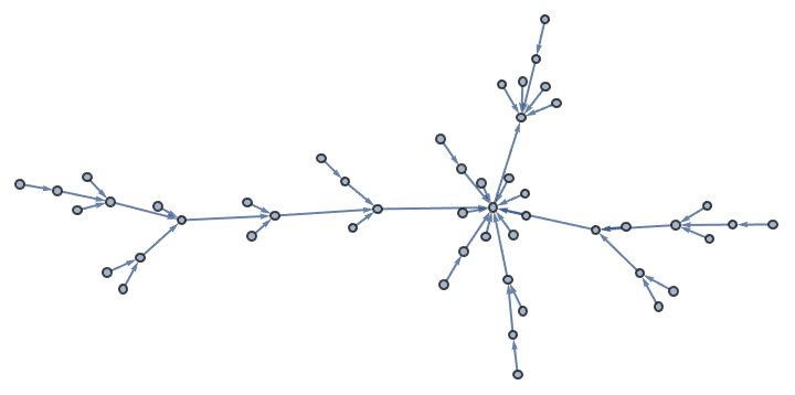
indegseq = VertexInDegree[g];
outdegseq = VertexOutDegree[g];IGRealizeDegreeSequence[outdegseq, indegseq]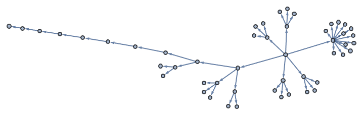
Verify that the degrees sequences of the result match the input to the function.
{VertexOutDegree[%] == outdegseq, VertexInDegree[%] == indegseq}{False, False}
S. L. Hakimi, On Realizability of a Set of Integers as Degrees of the Vertices of a Linear Graph, Journal of the Society for Industrial and Applied Mathematics 10, 3 (1962). http://eudml.org/doc/19050
V. Havel, Poznámka O Existenci Konečných Grafů (A Remark on the Existence of Finite Graphs), Časopis Pro Pěstování Matematiky 80, 4 (1955). https://www.jstor.org/stable/2098746
D. J. Kleitman and D. L. Wang, Algorithms for Constructing Graphs and Digraphs with Given Valences and Factors, Discrete Mathematics 6, 1 (1973). https://doi.org/10.1016/0012-365X(73)90037-X
Sz. Horvát and C. D. Modes, Connectivity matters: Construction and exact random sampling of connected graphs (2020). https://arxiv.org/abs/2009.03747
?IGGraphAtlas
This function is provided for convenience for those who have the book An Atlas of Graphs by Ronald C. Read and Robin J. Wilson, and for those who wish to replicate results obtained with other packages that include this database. For all other purposes, use Mathematica’s built-in GraphData function.
Retrieve graph number 789:
IGGraphAtlas[789]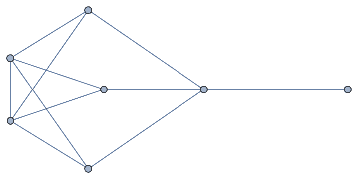
?IGFamousGraph
This function returns various “named” graphs from the igraph C
library’s built-in database. It is included in IGraph/M for
compatibility with other igraph interfaces. It is recommended to use
Mathematica’s built-in GraphData function instead. See the
documentation of the igraph C library for the list of supported graph
names.
Create Krackhardt’s kite graph:
g = IGFamousGraph["Krackhardt_Kite"]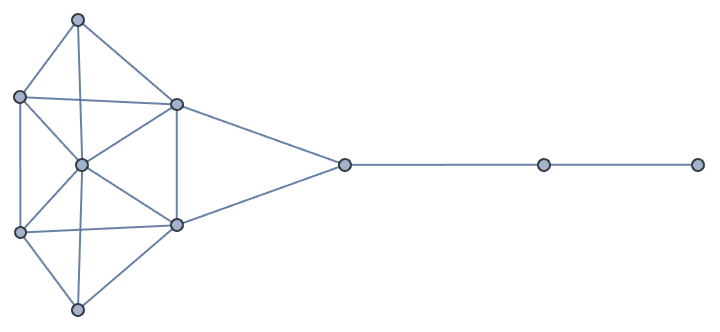
Krackhardt’s kite was devised to illustrate the difference between various centrality measures:
#[g] & /@ {
  IGVertexMap[0.1 # &, VertexSize -> IGBetweenness],
  IGVertexMap[# &, VertexSize -> IGCloseness],
  IGVertexMap[# &, VertexSize -> IGHarmonicCentrality],
  IGVertexMap[0.1 # &, VertexSize -> VertexDegree]
  }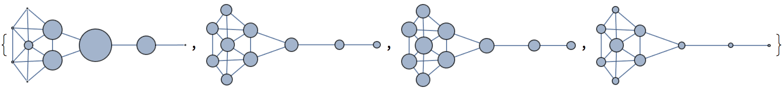
?IGFromNauty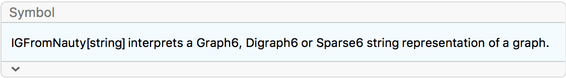
IGFromNauty converts a Graph6, Digraph6 or Sparse6
string to a graph. These formats originate with the nauty suite of programs and
are supported by many other graph theory software.
Interpret a Graph6 string.
IGFromNauty["Gr`HOk"]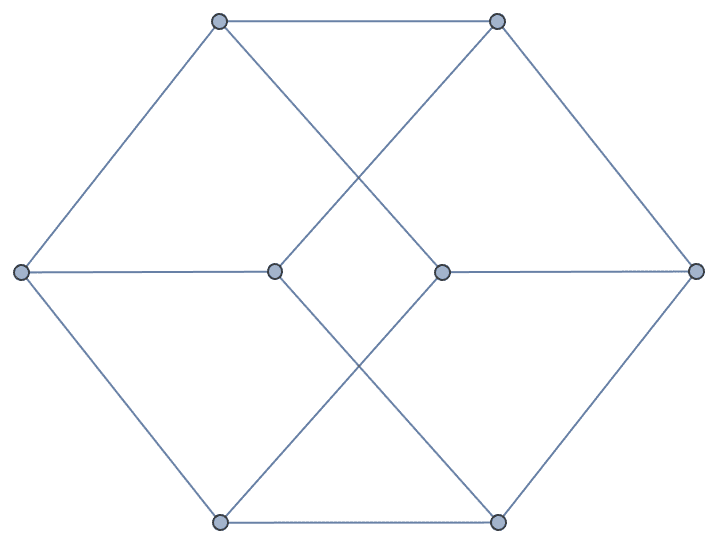
Interpret a Sparse6 string. These start with a :
character.
IGFromNauty[":I`ESgTlVF"]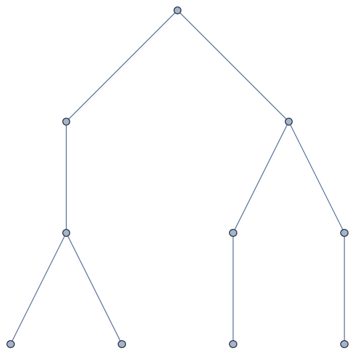
Interpret a Digraph6 string. These start with a &
character.
IGFromNauty["&FKB?oMB_W?"]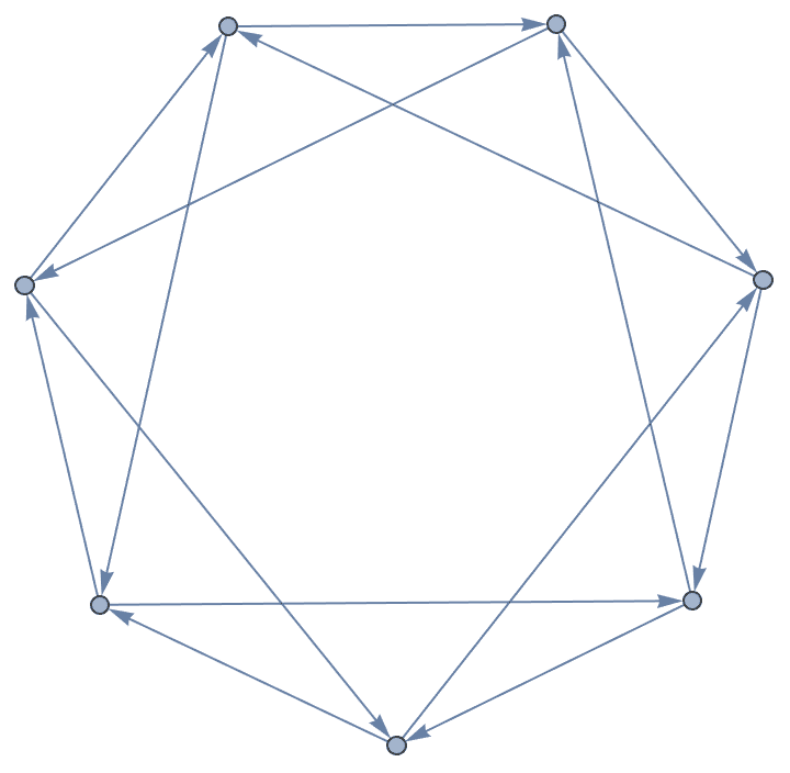
IGFromNauty does not support headers or whitespace in
the string. To handle these, or to interpret a multiline string, use
IGImportString[…, "Nauty"].
IGFromNauty[">>graph6<<DYw"]![]()
$Failed
IGImportString[
 ">>graph6<<DYw
Dhs
Dxo
DVW
", "Nauty"]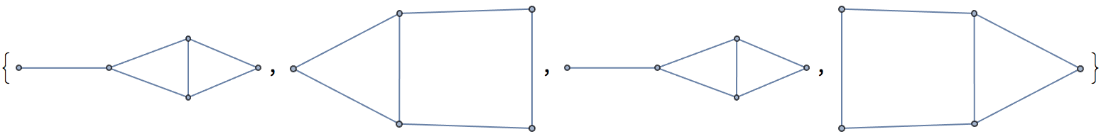
These graph creation functions use igraph’s random graph generator,
which can be seeded using IGSeedRandom.
?IG*Game*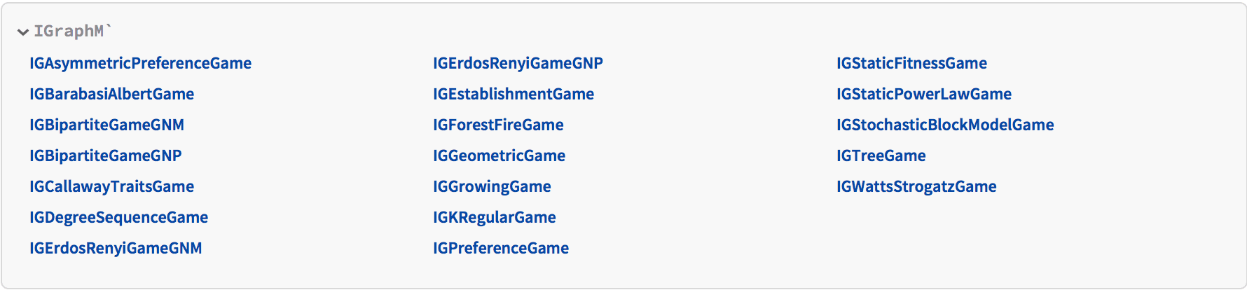
?IGErdosRenyiGameGNM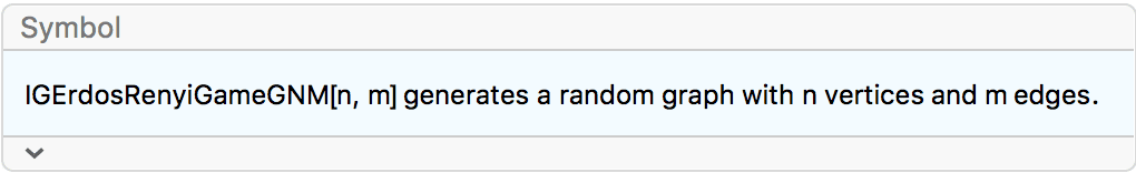
?IGErdosRenyiGameGNP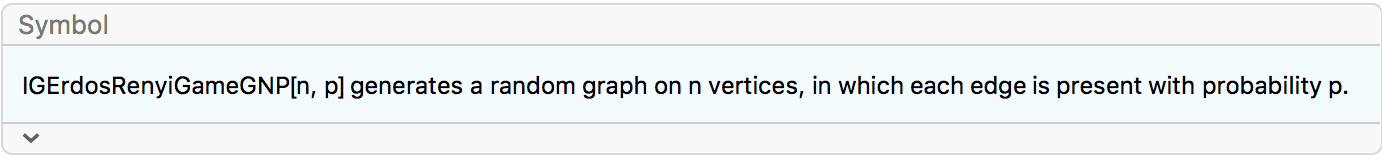
IGErdosRenyiGameGNM uniformly samples graphs with \(n\) vertices and \(m\) edges. This random graph model is known
as the Erdős–Rényi \(G(n,m)\)
model.
In IGErdosRenyiGameGNP, each edge is present with the
same and independent probability. This model is known as the Erdős–Rényi
\(G(n,p)\) model or Gilbert model.
The available options are:
DirectedEdges -> True produces a directed
graph.
SelfLoops -> True allows self-loops.
Create a random graph with 10 vertices and 20 edges.
IGErdosRenyiGameGNM[10, 20, GraphStyle -> "VintageDiagram"]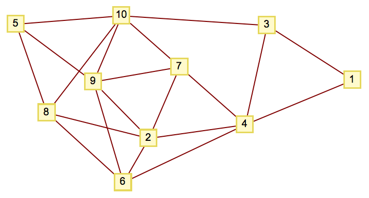
Create a directed graph and allow self-loops.
IGErdosRenyiGameGNM[10, 35, DirectedEdges -> True, SelfLoops -> True]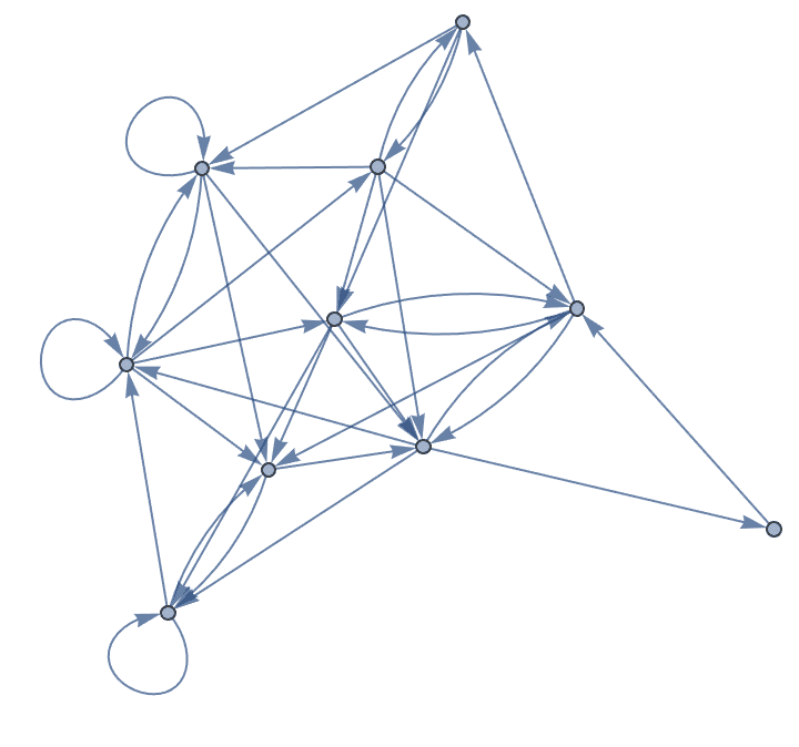
Insert each edge with a probability of 20%.
IGErdosRenyiGameGNP[20, 0.2, GraphStyle -> "RoyalColor"]
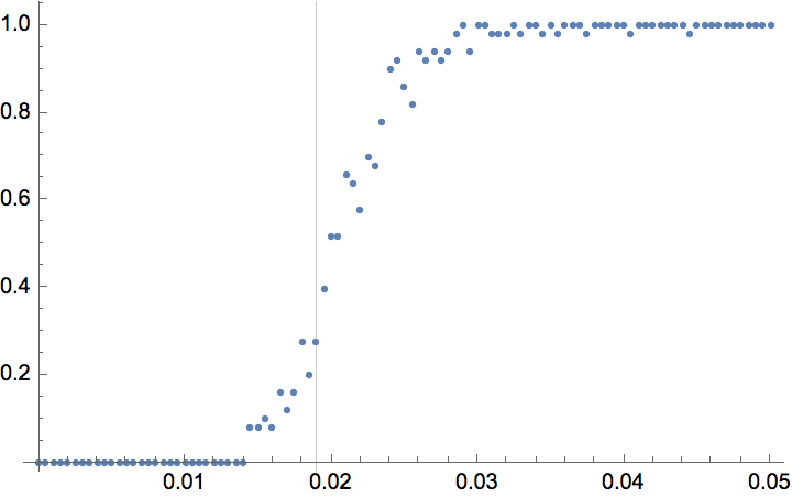
The \(G(n,p)\) model produces connected graphs with high probability for \(p>\ln (n)/n\).
n = 300;
ListPlot[
 Table[
  {p, Mean@
    Boole@Table[ConnectedGraphQ@IGErdosRenyiGameGNP[n, p], {50}]},
  {p, 0, 0.05, 0.0005}
  ],
 GridLines -> {{Log[n]/n}, None}
 ]
?IGBipartiteGameGNM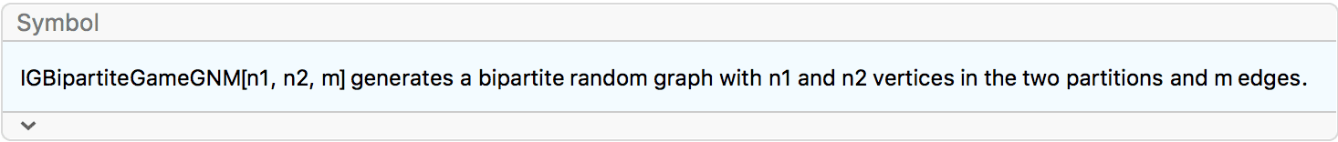
?IGBipartiteGameGNP
IGBipartiteGameGNM and IGBipartiteGameGNP
are equivalent to IGErdosRenyiGNM and
IGErdosRenyiGNP, but they generate bipartite graphs.
The available options are:
DirectedEdges -> True creates a directed
graph.
"Bidirectional" -> True allows directed edges to
run in either direction between the two partitions. The default is
False, which means that edges will run only from the first
partition to the second. This option is ignored for undirected
graphs.
IGBipartiteGameGNP[5, 5, 0.5, VertexLabels -> "Name"]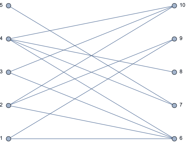
Create a bipartite directed graph with edges running either uni-directionally or bidirectionally between the two partitions.
IGLayoutBipartite@
   IGBipartiteGameGNM[10, 10, 30, DirectedEdges -> True,
    "Bidirectional" -> #] & /@ {False, True}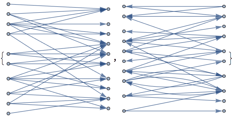
?IGTreeGame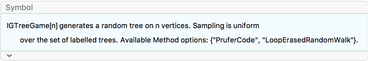
IGTreeGame samples uniformly from the set of labelled
trees.
Available options:
DirectedEdges -> True will create a directed
tree, with edges oriented away from the root.
Method can be used to choose the tree generation
algorithm. All methods sample labelled trees uniformly.
Available Method options:
"PruferCode", works by generating a random Prüfer
sequence, then constructing a tree from it. It does not currently
support directed trees.
"LoopErasedRandomWalk", uses a loop-erased random
walk to uniformly sample the spanning trees of the complete
graph.
IGTreeGame[250, GraphLayout -> "LayeredEmbedding",
 PlotTheme -> "PastelColor"]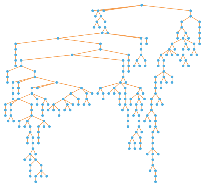
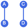
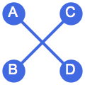
There are several distinct labellings of isomorphic trees. All of these are generated with equal probability.
Table[
  IGTreeGame[3, VertexLabels -> Automatic],
  {100}
] // DeleteDuplicatesBy[AdjacencyMatrix]![]()
Generate directed trees.
Table[IGTreeGame[6, DirectedEdges -> True,
  GraphLayout -> "LayeredDigraphEmbedding"], {5}]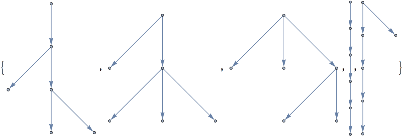
Generate a random sparse connected graph by first creating a tree, then adding cycle edges. Note that this method does not sample connected graphs uniformly.
randomConnected[nodeCount_, edgeCount_] :=
 Module[{tree},
  tree = IGTreeGame[nodeCount];
  EdgeAdd[tree,
   RandomSample[EdgeList@GraphComplement[tree],
    edgeCount - nodeCount + 1]]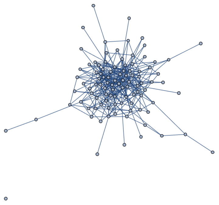
]randomConnected[100, 120]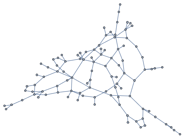
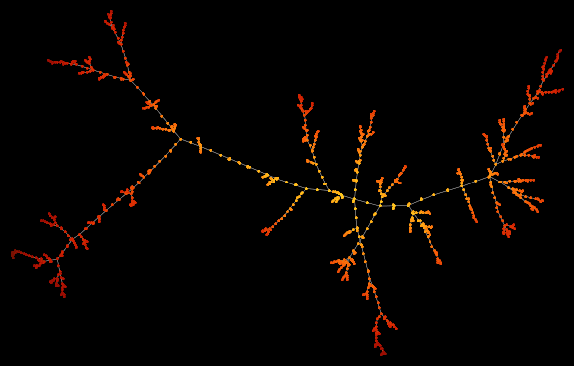
Colour the nodes of a random tree by their inverse average distance to other nodes.
IGVertexMap[
 ColorData["SolarColors"],
 VertexStyle -> Rescale@*IGCloseness,
 IGTreeGame[1000, Background -> Black, ImageSize -> Large,
  EdgeStyle -> LightGray]
 ]
?IGDegreeSequenceGame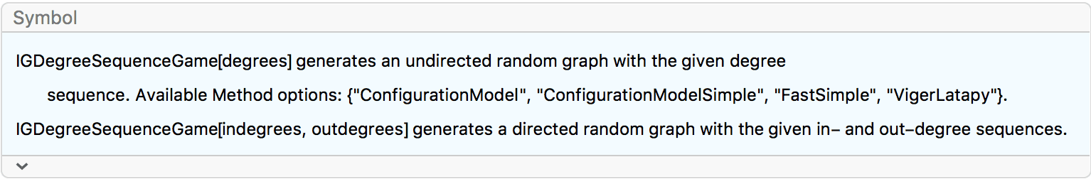
IGDegreeSequenceGame implements various random sampling
methods for graphs with a given degree sequence. To quickly construct a
single realization of a degree sequence, use
IGRealizeDegreeSequence.
IGDegreeSequenceGame takes the following values for its
Method option:
"ConfigurationModel" implements the configuration
model: it connects up vertex stubs randomly. It may generate both
self-loops and multi-edges. Undirected graphs are generated with
probability proportional to \(\left(\prod
_{i<j}A_{ij}!\prod _iA_{ii}\text{!!}\right){}^{-1}\), where
\(A\) is the adjacency matrix, having
twice the number of loops for each vertex on the diagonal.
Directed ones are generated with probability proportional to \(\left(\prod
_{i,j}A_{ij}!\right){}^{-1}\).
All simple graphs are generated with the same probability, but the probability of multigraphs and graphs with self-loops differs from that of simple graphs and depends on their specific structure.
"ConfigurationModelSimple" also implements the
configuration model, but it rejects non-simple graphs. It samples
uniformly from the set of all simple graphs with the given degree
sequence. This method can be very slow for dense graphs.
"FastSimple" is a fast generation algorithm that
avoids self-loops and multi-edges. This method can generate any simple
graph with the given degree sequence, but it does not sample them
uniformly.
"VigerLatapy" can sample undirected, connected
simple graphs uniformly and uses Monte-Carlo methods to randomize the
graphs. This generator should be favoured if undirected and connected
graphs are to be generated and execution time is not a concern. igraph
uses the original implementation of Fabien Viger; see https://www-complexnetworks.lip6.fr/~latapy/FV/generation.html
and the corresponding paper at https://arxiv.org/abs/cs/0502085.
The default method is "FastSimple". Note that it does
not sample uniformly.
degseq = VertexDegree@RandomGraph[{50, 100}];IGDegreeSequenceGame[degseq, Method -> "ConfigurationModel"]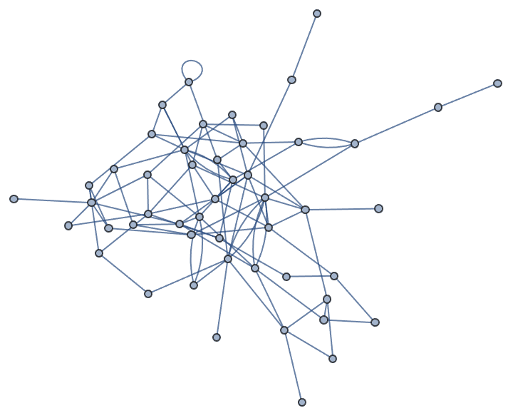
SimpleGraphQ[%]False
IGDegreeSequenceGame[degseq, Method -> "ConfigurationModelSimple"]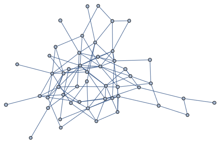
SimpleGraphQ[%]True
The configuration model algorithm is too slow to construct even small dense graphs.
ds = VertexDegree@RandomGraph[{10, Binomial[10, 2] - 5}]{9, 7, 7, 9, 9, 8, 8, 7, 8, 8}
TimeConstrained[
 IGDegreeSequenceGame[ds, Method -> "ConfigurationModelSimple"], 1]
$Aborted
Graphs that are almost complete can be sampled by generating the complement first.
GraphComplement@
IGDegreeSequenceGame[9 - ds, Method -> "ConfigurationModelSimple"]![]()
ds == VertexDegree[%]True
?IGKRegularGame
In a \(k\)-regular graph all vertices have degree \(k\). The current implementation is able to generate any \(k\)-regular graph, but it does not sample them with precisely the same probability.
The available options are:
DirectedEdges -> True creates a directed
graph.
MultiEdges -> True allows the creation of
parallel edges.
IGKRegularGame[10, 3]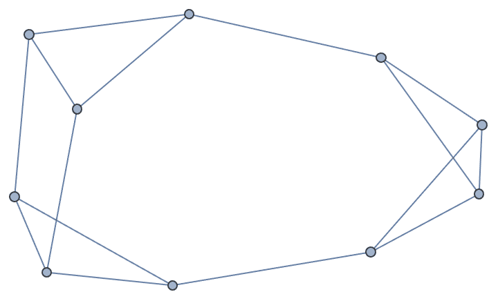
Not all parameters are valid:
IGKRegularGame[5, 3]![]()
![]()
$Failed
There are no graphs with 5 vertices each having degree 3.
IGGraphicalQ[{3, 3, 3, 3, 3}]False
?IGGrowingGame
IGGrowingGame[n, k] creates a random graph by
successively adding vertices to the graph until the vertex count
n is reached. At each step, k new edges are
added as well.
The available options are:
DirectedEdges -> True creates a directed
graph.
"Citation" -> True connects newly added edges to
the newly added vertex.
IGGrowingGame[50, 2]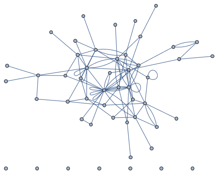
With "Citation" -> True, the newly added edges are
connected to the newly added vertices.
IGGrowingGame[50, 1, "Citation" -> True]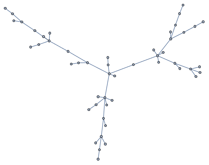
Note that while this model can be used to generate random trees, it
will not sample them uniformly. If uniform sampling is desired, use
IGTreeGame instead.
Create a directed citation graph.
IGGrowingGame[20, 2, DirectedEdges -> True, "Citation" -> True,
 GraphStyle -> "Web"]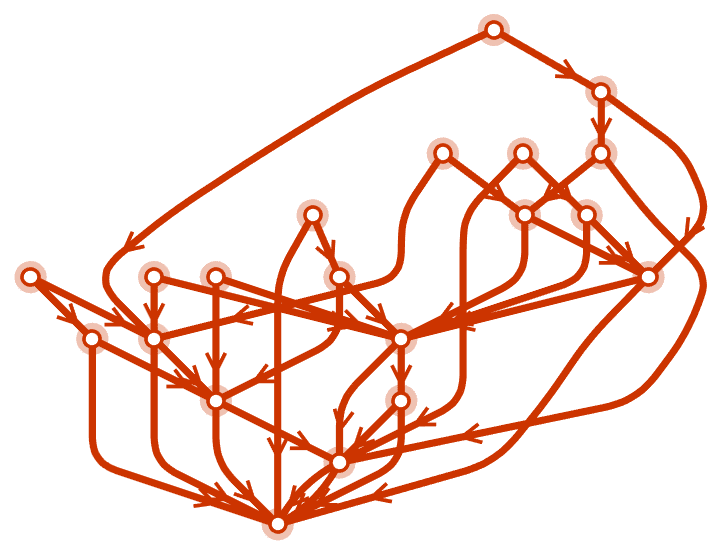
?IGBarabasiAlbertGame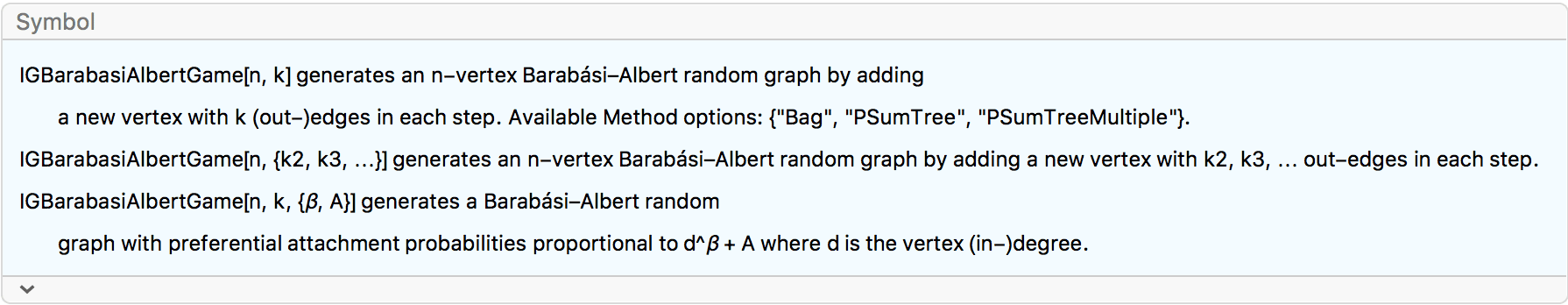
IGBarabasiAlbertGame implements a preferential
attachment model. It generates a graph by sequentially adding new
vertices with the specified number of edges (\(k\)). The edges will connect to existing
vertices with probability \(d^{\beta
}+A\), where \(d\) is the
in-degree of the existing vertex. The default parameters are \(\beta =1\) and \(A=1\).
The available options are:
DirectedEdges -> False creates an undirected
graph.
"TotalDegreeAttraction" -> True computes the
attachment probability based on the the total degree of existing
vertices (i.e. the sum of in- and out-degrees), not their in-degree.
Always assumed to be True when using
DirectedEdges -> True.
"StartingGraph" -> g will use graph
g as the starting point for building the preferential
attachment graph. The vertex names of g are ignored; the
result always uses positive integers as vertex names.
Available Method option values:
"Bag" works by putting the IDs of the vertices into
a bag exactly as many times as their (in-)degree, plus once more. Then
the required number of cited vertices are drawn from the bag, with
replacement. This method might generate multi-edges. It only works if
\(\beta =1\) and \(A=1\).
"PSumTree" uses a partial prefix-sum tree to
generate the graph. It does not generate multi-edges and works for any
\(\beta\) and \(A\) values.
"PSumTreeMultiple" works like
"PSumTree" but allows multi-edges.
The built-in BarabasiAlbertGraphDistribution is
equivalent to using \(A=0\) and
DirectedEdges -> False in
IGBarabasiAlbertGame, while the built-in
PriceGraphDistribution is equivalent
DirectedEdges -> True.
IGBarabasiAlbertGame[100, 1]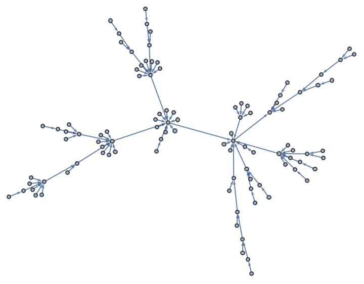
Use attachment probability proportional to
degree^1.5 + 1.
IGBarabasiAlbertGame[100, 2, {1.5, 1}]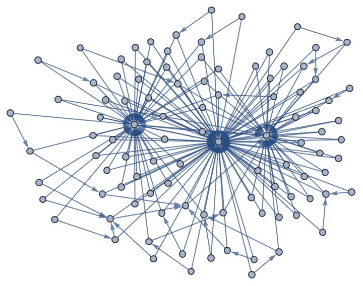
The "Bag" method may generate parallel edges:
IGBarabasiAlbertGame[100, 2, Method -> "Bag"]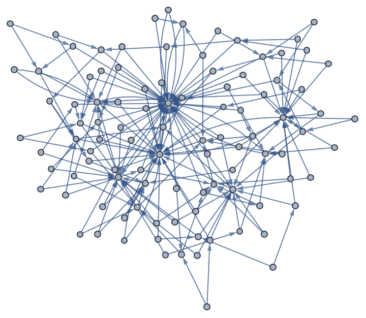
MultigraphQ[%]True
Create a graph with the given out-degree sequence. The \(k^{\text{th}}\) entry in the degree sequence list must be no greater than \(k\).
IGBarabasiAlbertGame[12, {1, 2, 3, 2, 1, 3, 4, 5, 1, 5, 2},
 PlotTheme -> "Minimal"]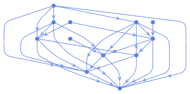
VertexOutDegree[%]{0, 1, 2, 3, 2, 1, 3, 4, 5, 1, 5, 2}
Create a preferential attachment graph using a 4-node complete graph as the starting point.
IGBarabasiAlbertGame[10, 1, "StartingGraph" -> CompleteGraph[4]]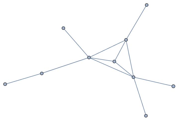
?IGWattsStrogatzGame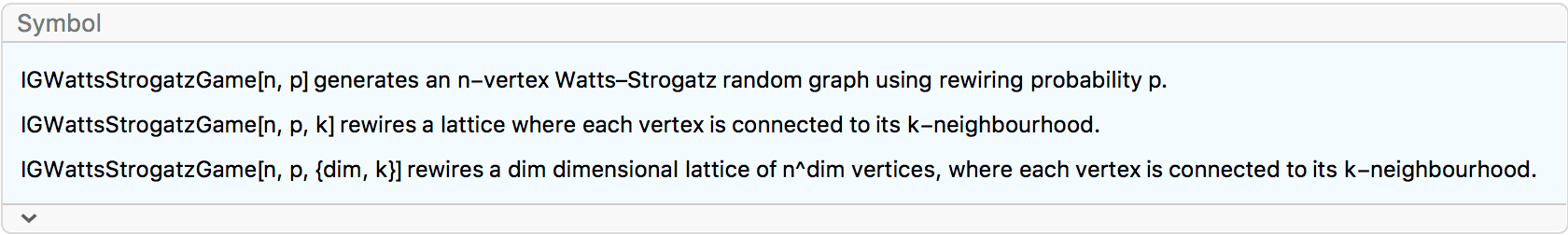
The two-argument form produces results equivalent to that of the
built-in WattsStrogatzGraphDistribution.
IGWattsStrogatzGame[30, 0.05, PlotTheme -> "Web"]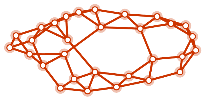
The extended form allows for multi-dimensional lattices. Create a graph by randomly rewiring a two-dimensional toroidal lattice of \(10\times 10\) nodes:
Graph3D@IGWattsStrogatzGame[10, 0.01, {2, 1}]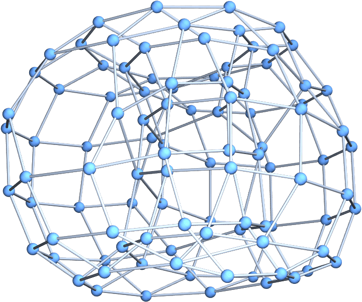
?IGStaticFitnessGame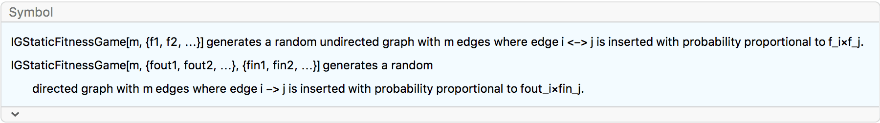
IGStaticFitnessGame generates a random graph by
connecting vertices based on their fitness score. The algorithm starts
with \(n\) vertices and no edges. Two
vertices are selected with probabilities proportional to their fitness
scores (for directed graphs, a starting vertex is selected based on its
out-fitness and an end vertex based on its in-fitness). If they are not
yet connected, an edge is inserted between them. The procedure is
repeated until the number of edges reaches \(m\).
The expected degree of each vertex is proportional to its fitness score. This is exactly true when self-loops and multi-edges are allowed, and approximately true otherwise.
IGStaticFitnessGame approximates the Chung–Lu model in
which each edge i <-> j is present independently,
with probability
\[p_{ij}= \begin{array}{ll} \{ & \begin{array}{ll} \frac{f_if_j}{2m} & \text{if} i\neq j \\ \frac{f_if_j}{4m} & \text{if} i=j \\ \end{array} \\ \end{array} ,\]
where \(m=\frac{1}{2}\sum _kf_k\).
Unlike the Chung–Lu algorithm, which would require \(O\left(m^2\right)\) computation steps,
IGStaticFitnessGame runs in \(O(m)\) time.
The available options are:
SelfLoops -> True allows the creation of
self-loops.
MultiEdges -> True allows the creation of
parallel edges.
Create an undirected graph with four high-degree nodes and 40 low-degree ones.
weights = Join[{10, 10, 10, 10}, ConstantArray[1, 40]];
IGStaticFitnessGame[Total[weights]/2, weights]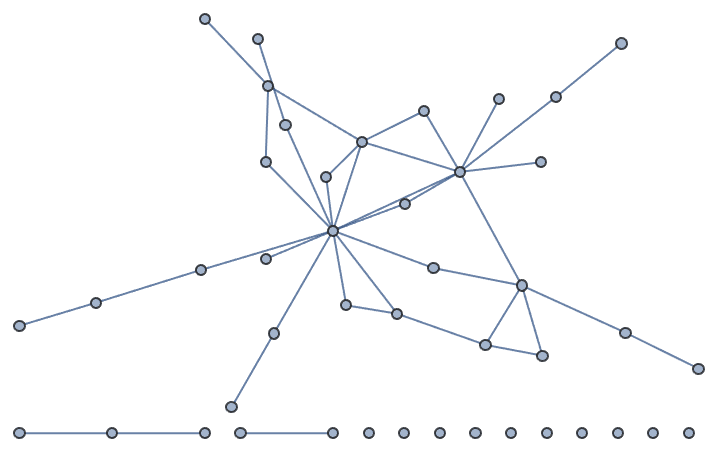
VertexDegree[%]{5, 5, 12, 8, 2, 2, 1, 2, 2, 1, 1, 2, 2, 0, 2, 1, 2, 0, 0, 3, 1, 1, \ 0, 0, 1, 2, 0, 3, 0, 2, 1, 2, 1, 1, 1, 2, 0, 1, 2, 0, 0, 3, 2, 1}
Create a directed graph.
IGStaticFitnessGame[30, Range[10], Range[10, 1, -1]]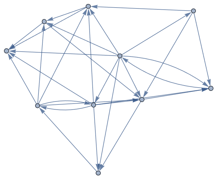
When self-loops and multi-edges are allowed, the expected degree of each vertex is proportional to its fitness score.
degrees = {3, 3, 2, 2, 2, 1, 1};
Table[
   VertexDegree@IGStaticFitnessGame[
     Total[degrees]/2, degrees,
     SelfLoops -> True, MultiEdges -> True
     ],
   {1000}
] // N // Mean{3.03, 2.97, 2.023, 1.957, 2.056, 0.977, 0.987}
When generating simple graphs, this holds only approximately.
degrees = {3, 3, 2, 2, 2, 1, 1};
Table[
   VertexDegree@IGStaticFitnessGame[
     Total[degrees]/2, degrees
     ],
   {1000}
] // N // Mean{2.703, 2.625, 2.04, 2.071, 2.086, 1.23, 1.245}
?IGStaticPowerLawGame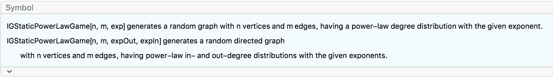
IGStaticPowerLawGame generates a directed or undirected
random graph where the degrees of vertices follow power-law
distributions with prescribed exponents. For directed graphs, the
exponents of the in- and out-degree distributions may be specified
separately.
This function is equivalent to IGStaticFitnessGame with
a fitness vector \(f\) where \(f_i=i^{-\alpha }\) and \(\alpha =\frac{1}{\text{exponent}-1}\).
Note that significant finite size effects may be observed for exponents smaller than 3 in the original formulation of the game. This function removes the finite size effects by default by assuming that the fitness of vertex \(i\) is \(\left(i+i_0\right){}^{-\alpha }\), where \(i_0\) is a constant chosen appropriately to ensure that the maximum degree is less than the square root of the number of edges times the average degree; see the paper of Chung and Lu, and Cho et al. for more details.
The available options are:
SelfLoops -> True allows the creation of
self-loops.
MultiEdges -> True allows the creation of
parallel edges.
"FiniteSizeCorrection" -> False disables finite
size correction, which is used by default.
Create a graph with a power-law degree distribution of exponent 2.5.
g = IGStaticPowerLawGame[100000, 200000, 2.5];Histogram[VertexDegree[g], "Log", {"Log", "PDF"}]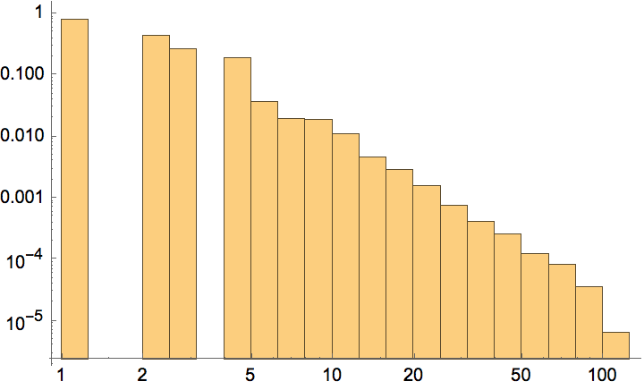
Create a directed graph with power-law in- and out-degree distributions.
IGStaticPowerLawGame[50, 150, 3, 3]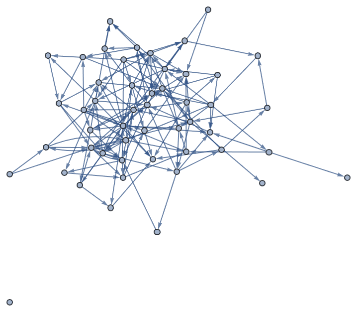
Goh K-I, Kahng B, Kim D: Universal behaviour of load distribution in scale-free networks. Phys Rev Lett 87(27):278701, 2001.
Chung F and Lu L: Connected components in a random graph with given degree sequences. Annals of Combinatorics 6, 125-145, 2002.
Cho YS, Kim JS, Park J, Kahng B, Kim D: Percolation transitions in scale-free networks under the Achlioptas process. Phys. Rev. Lett. 103:135702, 2009.
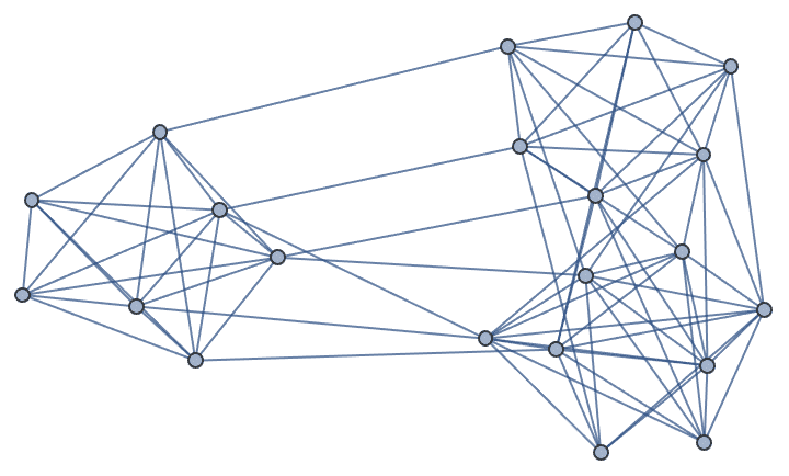
?IGStochasticBlockModelGame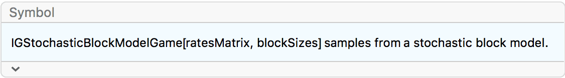
The ratesMatrix argument gives the connection
probability between and within blocks (groups of vertices). The
blockSizes argument gives the size of each block (vertex
group).
The available options are:
DirectedEdges -> True creates a directed
graph.
SelfLoops -> True allows the creation of
self-loops.
![]()
IGAdjacencyMatrixPlot[%]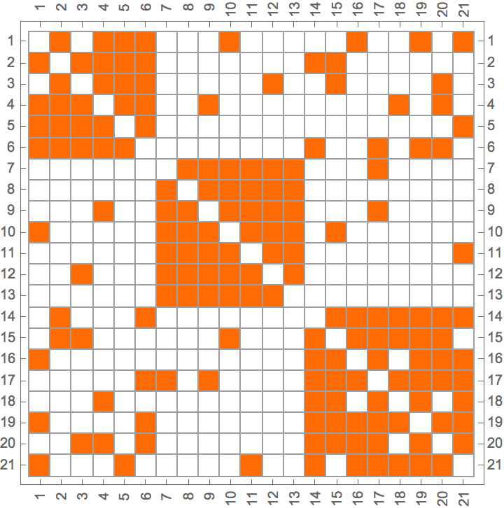
?IGPreferenceGame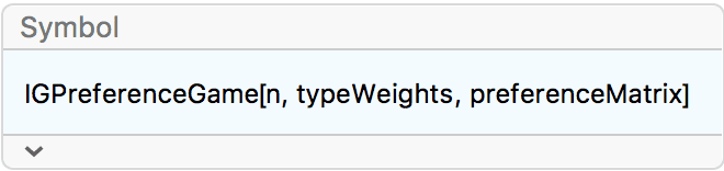
Experimental: This is experimental functionality that may change without notice.
IGPreferenceGame[n, w, p] first samples n
vertices of different types, each having type \(i\) with probability proportional to \(w_i\). Then it connects vertices with types
\(i\) and \(j\) with probability \(p_{ij}\). This is similar to a stochastic
block model, but the vertex types are chosen randomly.
The available options are:
DirectedEdges -> True creates a directed
graph.
SelfLoops -> True allows self-loops.
Generate a graph with three groups of vertices of different sizes, with intra-group connections being much more frequent than inter-group ones.
IGPreferenceGame[60, {3, 6, 10}, 0.05 + 0.5 IdentityMatrix[3]]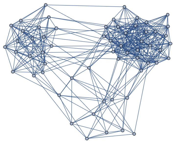
Generate a directed graph with low-probability intra-group connections and high probability unidirectional inter-group connections.
![]()
?IGAsymmetricPreferenceGame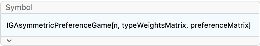
Experimental: This is experimental functionality that may change without notice.
IGAsymmetricPreferenceGame[n, w, p] is similar to
IGPreferenceGame[n, w, p], but it assigns a separate
out-type and in-types to each vertex. The probability of a vertex having
out-type \(i\) and in-type \(j\) is proportional to \(w_{ij}\). The probability of connecting a
vertex with out-type \(i\) to another
one with in-type \(j\) is \(p_{ij}\).
The available options are:
SelfLoops -> True allows self-loops.![]()
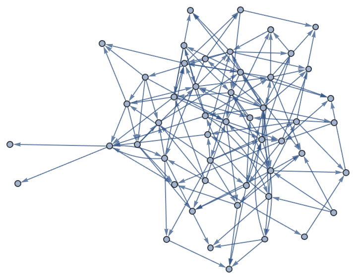
?IGForestFireGame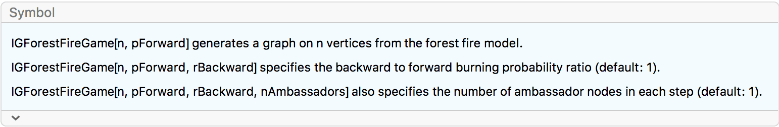
The forest fire model is a growing graph model. In every time step, a
new vertex is added to the graph. The new vertex chooses the specified
number of ambassadors (default: 1) and starts a simulated forest fire at
their locations. The fire spreads through the directed edges. The
spreading probability along an edge is given by pForward.
The fire may also spread backwards on an edge with probability
pForward * rBackward. When the fire has ended, the newly
added vertex connects to all the vertices that were burned in the
fire.
The forest fire model intends to reproduce the following network characteristics, observed in real networks:
Heavy-tailed in-degree and out-degree distributions.
Community structure.
Densification power-law. The network is densifying in time, according to a power-law rule.
Shrinking diameter. The diameter of the network decreases in time.
The available options are:
DirectedEdges -> False generates an undirected
graph.Generate a graph with only forward burning.
IGForestFireGame[30, 0.2, 0,
 GraphLayout -> "SpringEmbedding"]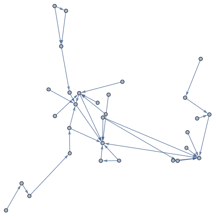
Generate a graph from the forest fire model, and visualize its community structure.
IGForestFireGame[100, 0.2, 1, 2, DirectedEdges -> False,
 GraphLayout -> {"EdgeLayout" -> "HierarchicalEdgeBundling"}]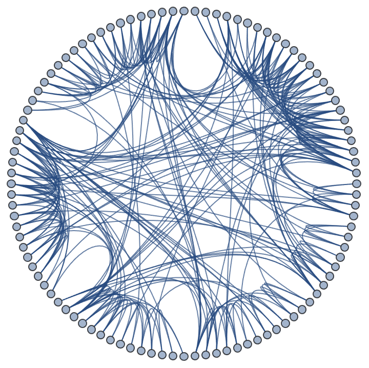
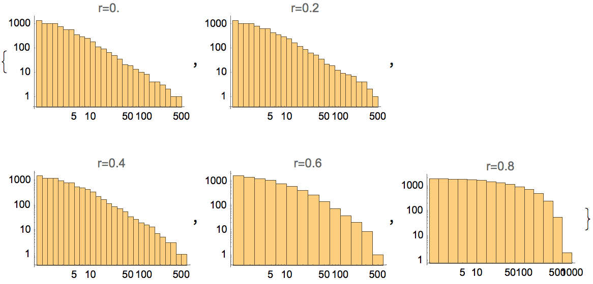
Plot the cumulative in-degree distribution for different backward to forward burning probability ratios.
Table[
 Histogram[
  VertexInDegree@
   IGForestFireGame[2000, 0.4, r, 2, DirectedEdges -> True],
  "Log", {"Log", "SurvivalCount"},
  PlotLabel -> Row[{"r=", r}]
  ],
 {r, 0, 0.8, 0.2}
 ]
Jure Leskovec, Jon Kleinberg and Christos Faloutsos. Graph
evolution: Densification and shrinking diameters.
ACM Transactions on Knowledge Discovery from Data (TKDD), 2007.
https://doi.org/10.1145/1217299.1217301
Jure Leskovec, Jon Kleinberg and Christos Faloutsos. Graphs over time: densification laws, shrinking diameters and possible explanations. KDD ’05: Proceeding of the eleventh ACM SIGKDD international conference on Knowledge discovery in data mining, 177–187, 2005.
?IGCallawayTraitsGame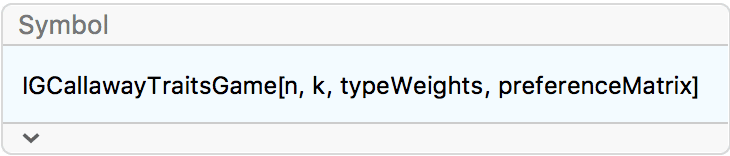
This function simulates a growing random graph according to the following algorithm:
At each time step, a new vertex is added. Its type is randomly
selected according to the type weights. Then k existing
pairs of vertices are selected randomly, and each pair attempts to
connect. The probability of success for given types of vertices is given
by the preference matrix.
This algorithm may create self-loops and multi-edges.
The available options are:
DirectedEdges -> True creates a directed graph.![]()
?IGEstablishmentGame
This function simulates a growing random graph according to the following algorithm:
At each time step, a new vertex is added. Its type is randomly
selected according to the type weights. It attempts to connect to
k distinct existing vertices. The probability of success
for given types of vertices is given by the preference matrix.
The available options are:
DirectedEdges -> True creates a directed graph.![]()
?IGGeometricGame
Available options:
"Periodic" -> True assumes a toroidal topologyIGGeometricGame[50, 0.2]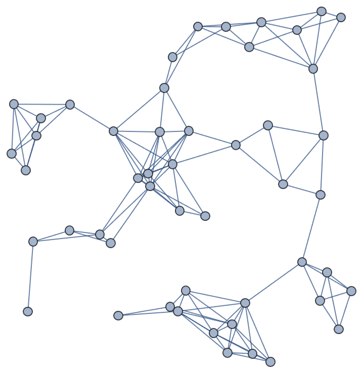
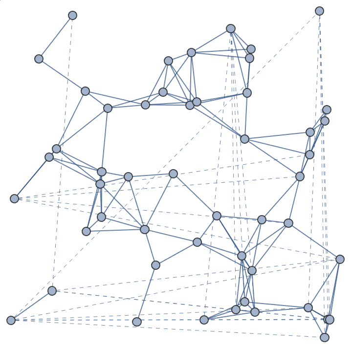
Use a toroidal topology and draw “wraparound” edges with dashed lines.
IGGeometricGame[50, 0.2, "Periodic" -> True] //
 IGEdgeMap[
  If[EuclideanDistance @@ # > 0.2, Dashed, None] &,
  EdgeStyle -> IGEdgeVertexProp[VertexCoordinates]
  ]
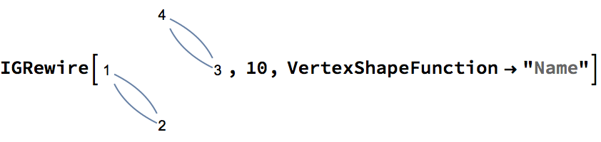
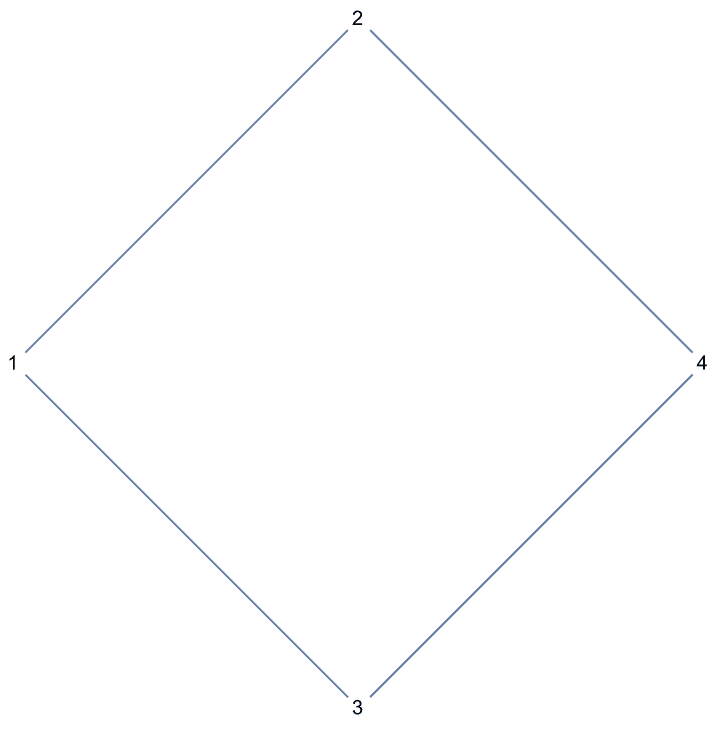
?IGRewire
IGRewire will try to rewire the edges of the graph the
given number of times by switching random pairs of edges as below, thus
preserving the graph’s degree sequence.
 ⟶
⟶
 or
⟶
or
⟶
The switches succeed only if they would not create multi-edges. The parameter \(n\) specifies the number of switch attempts, not the number of successful switches.
For directed graphs, the switches are such that they preserve both the in- and out-degree sequence.
The vertex ordering of the graph is retained.
Warning: Most graph properties, such as edge weights, will be lost.
The available options are:
SelfLoops -> True allows the creation of
self-loops.Generate a random network with scale-free degree distribution:
IGRewire[IGBarabasiAlbertGame[200, 2, DirectedEdges -> False], 10000]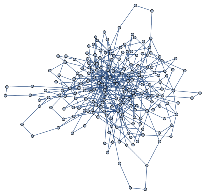
Use SelfLoops -> True to allow creating loops.
Table[IGRewire[PathGraph@Range[4], 100, SelfLoops -> True], {5}]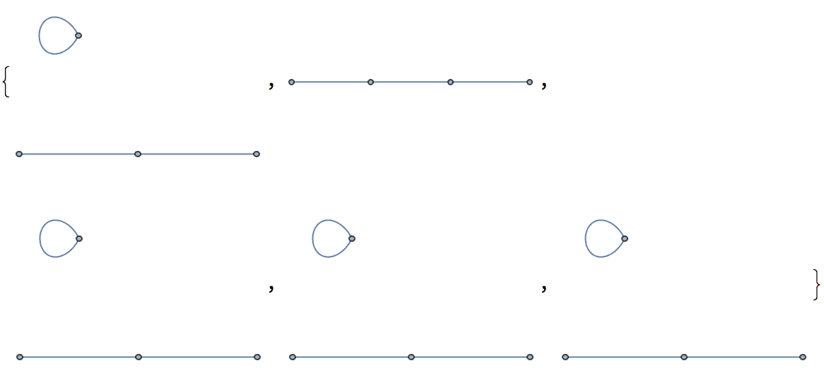
IGRewrire never creates any multi-edges. Multigraphs are
allowed as input, but a warning is given.
![]()
Uniformly sample simple labelled graphs with a given degree sequence by first creating a single realization, then rewiring it a sufficient amount of times.
degseq = {3, 3, 2, 2, 1, 1};Table[
IGRewire[IGRealizeDegreeSequence[degseq], 100],
{1000}
] // CountsBy[AdjacencyMatrix] // KeySort //
KeyMap[AdjacencyGraph[#, VertexShapeFunction -> "Name"] &]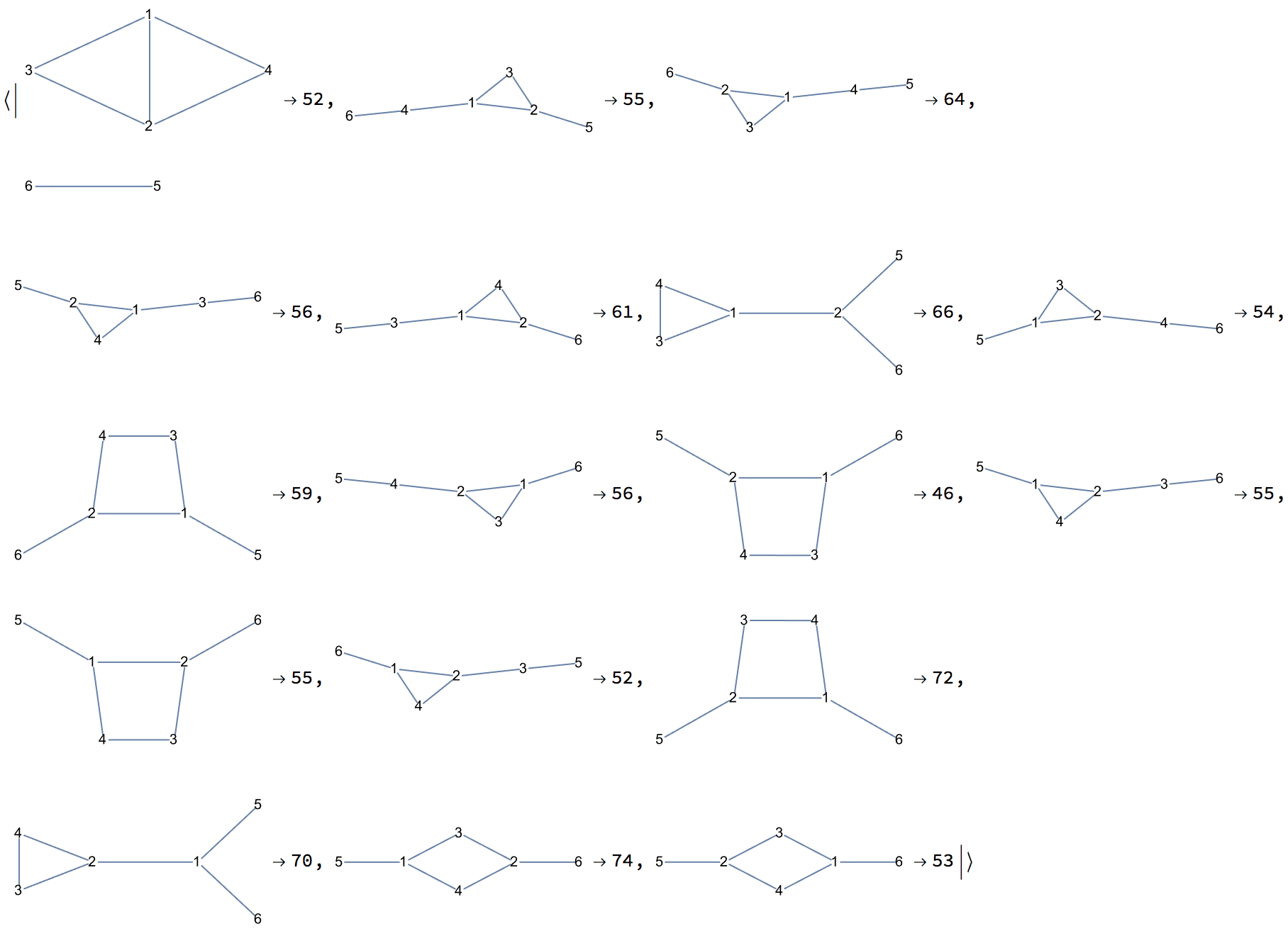
?IGRewireEdges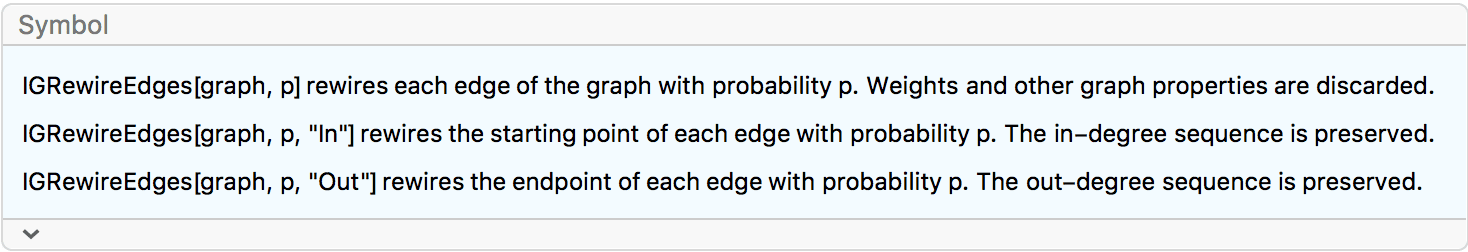
IGRewireEdges randomly rewires each edge of the graph
with the given probability. The vertex ordering is retained.
For directed graphs, it can optionally rewire only the starting point
or endpoint of directed edges, thus preserving the out- or in-degree
sequence. In this case, the MultiEdges option is ignored
and multi-edges may be created.
Warning: Most graph properties, such as edge weights, will be lost.
The available options are:
SelfLoops -> True allows the creation of
self-loops.
MultiEdges -> True allows the creation of
multi-edges.
Create a random graph with 10 vertices and 20 edges, while allowing for multi-edges:
IGRewireEdges[RandomGraph[{10, 20}], 1, MultiEdges -> True]
EdgeCount[%]20
Rewire the endpoint of each edge, preserving the out-degree sequence.
g = RandomGraph[{10, 30}, DirectedEdges -> True];
{VertexInDegree[g], VertexOutDegree[g]}{{5, 4, 1, 2, 2, 2, 5, 3, 3, 3}, {2, 6, 4, 2, 2, 4, 3, 2, 2, 3}}
rg = IGRewireEdges[g, 1, "Out"];
{VertexInDegree[rg], VertexOutDegree[rg]}{{2, 0, 2, 7, 3, 3, 3, 3, 2, 5}, {2, 6, 4, 2, 2, 4, 3, 2, 2, 3}}
Note that multi-edges were created.
MultigraphQ[rg]True
?IGVertexContract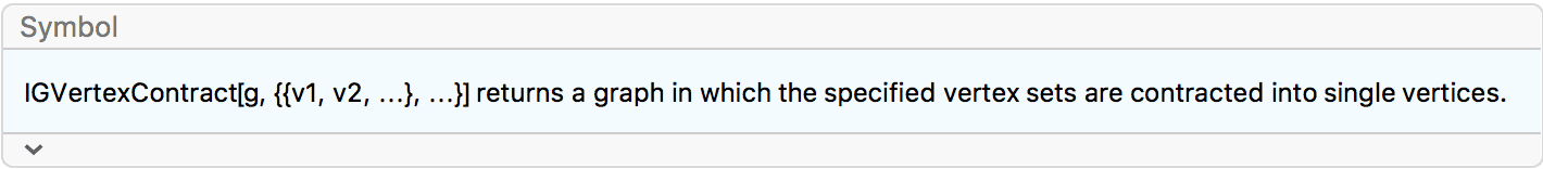
IGVertexContract[g, {set1, set2, …}] will simultaneously
contract multiple vertex sets into single vertices.
The name of a contracted vertex will be the same as the first element
of the corresponding set. Vertex ordering is not retained. Edge ordering
is retained only when using both
SelfLoops -> True and
MultiEdges -> True.
Warning: Most graph properties, such as edge weights, will be lost.
The available options are:
SelfLoops -> True keeps any self-loops created
during contraction.
MultiEdges -> True keeps any parallel edges
created during contraction.
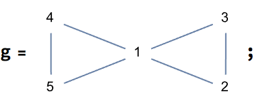
IGVertexContract[g, {{1, 2, 3}, {4, 5}}, VertexLabels -> "Name"]![]()
IGVertexContract[g, {{1, 2, 3}, {4, 5}}, SelfLoops -> True]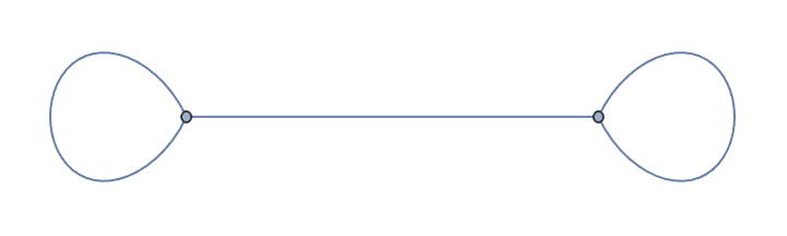
IGVertexContract[g, {{1, 2, 3}, {4, 5}}, SelfLoops -> True,
 MultiEdges -> True]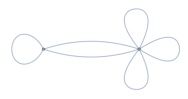
IGVertexContract[g, {{1, 2, 3}, {4, 5}}, MultiEdges -> True]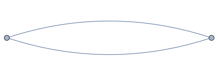
When using both SelfLoops -> True and
MultiEdges -> True, the edge ordering is maintained
relative to the input graph. This allows easily transferring edge
weights, and combining them if necessary.
g = IGShorthand["a-b-c-d-a,a-c",
  EdgeWeight -> {1, 2, 3, 4, 5}, EdgeLabels -> "EdgeWeight"]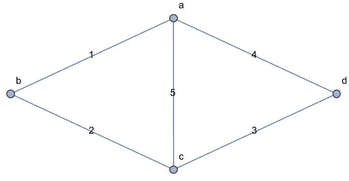
IGWeightedSimpleGraph[
 IGVertexContract[g, {{"a", "b"}},
  SelfLoops -> True, MultiEdges -> True,
  EdgeWeight -> IGEdgeProp[EdgeWeight][g]
  ],
 EdgeLabels -> "EdgeWeight", VertexLabels -> "Name"
 ]
?IGConnectNeighborhood
IGConnectNeighborhood[g, k] connects each vertex in
g to its order k neighbourhood. This operation
is also known as the \(k^{\text{th}}\)
power of the graph.
IGConnectNeighborhood differs from the built-in
GraphPower in that it preserves parallel edges and
self-loops.
Warning: Most graph properties, such as edge weights, will be lost.
Connect each vertex to its second order neighbourhood:
IGConnectNeighborhood[CycleGraph[15]]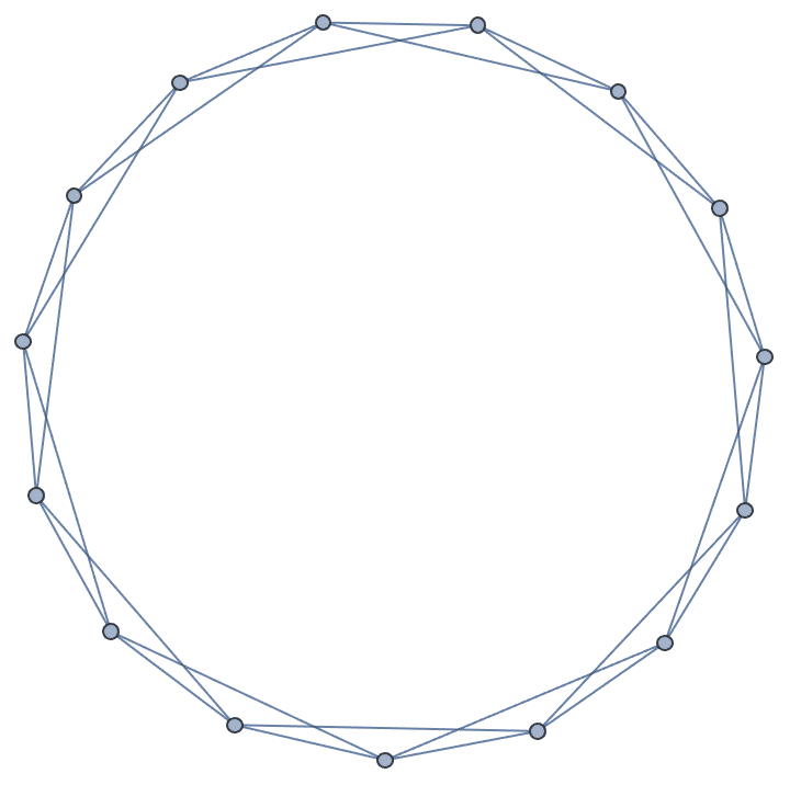
Connect each vertex to its third order neighbourhood:
IGConnectNeighborhood[GridGraph[{10, 10}], 3]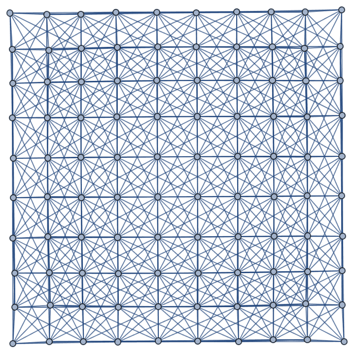
?IGMycielskian
IGMycielskian applies the Mycielski
construction to an undirected graph on \(n\geq 2\) vertices to obtain a larger graph
(the Mycielskian) on \(2 n+1\)
vertices. If the graph has less than 2 vertices, then instead of
applying the standard Mycielski construction, IGMycielskian
simply adds one vertex and one edge.
If the original graph has chromatic number \(k\), its Mycielskian has chromatic number \(k+1\). The Mycielski construction preserves the triangle-free property of the graph.
g = CycleGraph[4]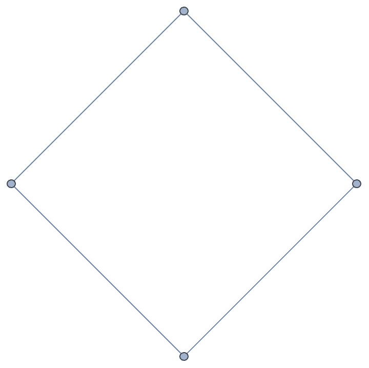
{IGChromaticNumber[g], IGTriangleFreeQ[g]}{2, True}
mg = IGMycielskian[g]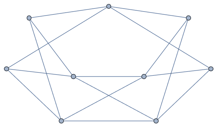
{IGChromaticNumber[mg], IGTriangleFreeQ[mg]}{3, True}
Construct triangle-free graphs with successively larger chromatic numbers.
NestList[IGMycielskian, IGEmptyGraph[], 5]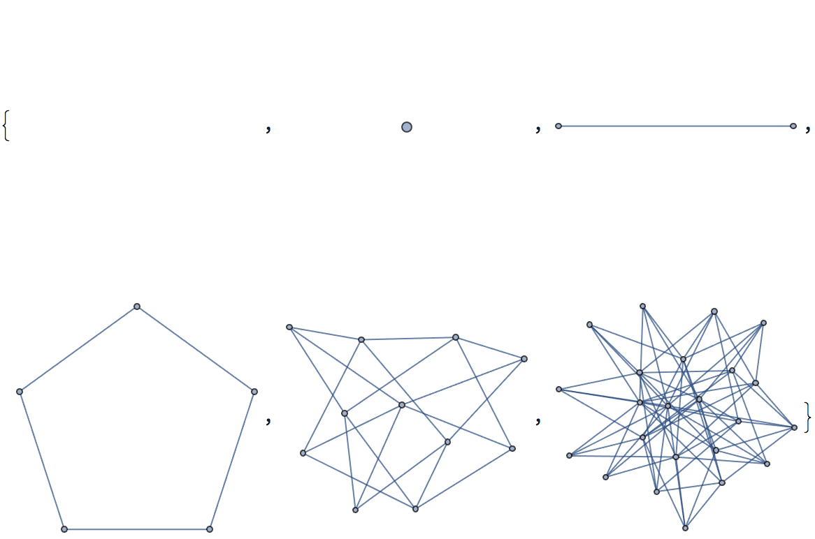
IGChromaticNumber /@ %{0, 1, 2, 3, 4, 5}
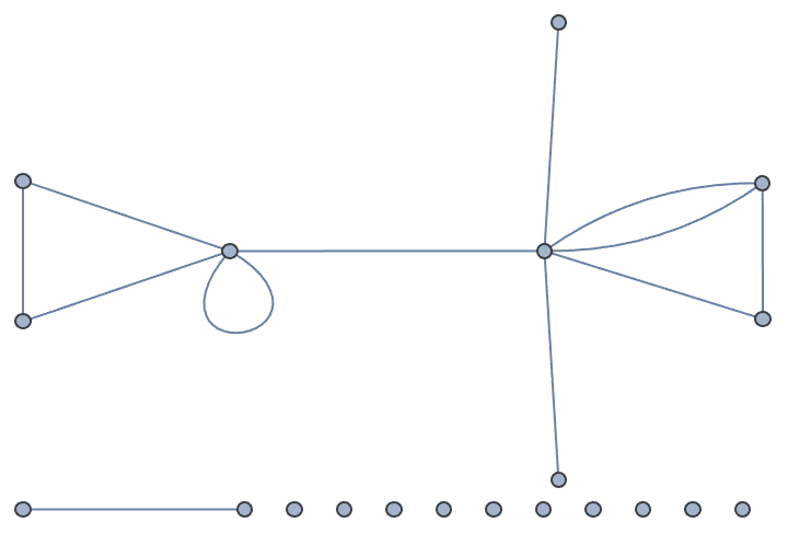
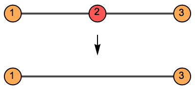
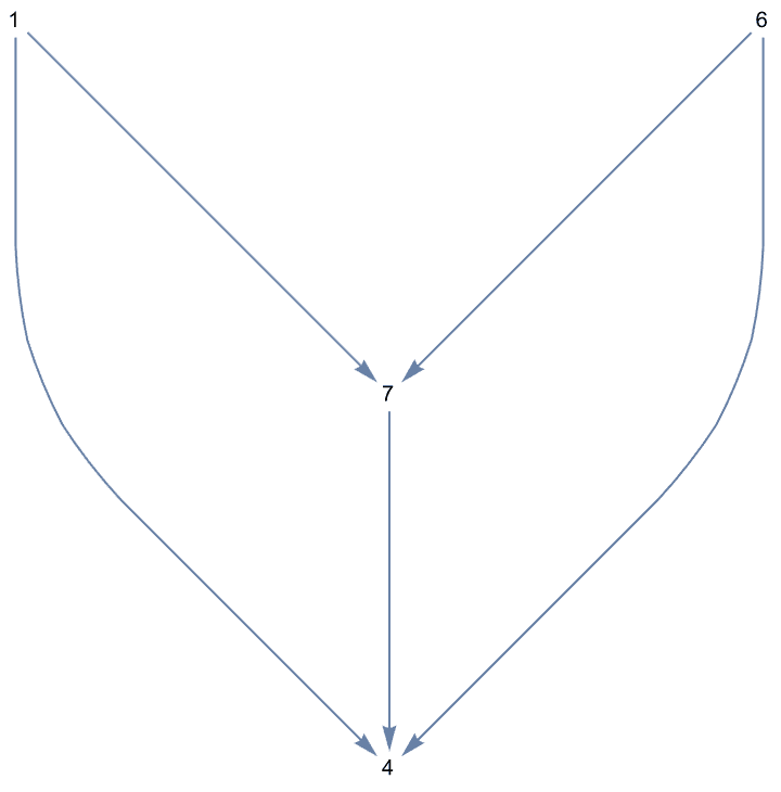
?IGSmoothen
IGSmoothen suppresses all degree-2 vertices, thus
obtaining the smallest topologically equivalent (i.e. homeomorphic)
graph. See also IGHomeomorphicQ.
![]()
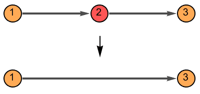
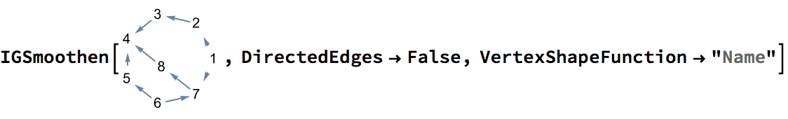
The vertex names are preserved, and the weights of merged edges are summed up. All other graph properties are discarded. In directed graphs, only those vertices are smoothened which have one incoming and one outgoing edge.
Available options:
DirectedEdges -> False ignores edge directions in
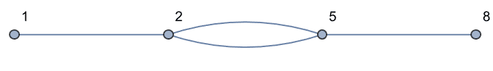
the input graph.The smallest topological equivalent of a path graph consists of two connected vertices.
![]()
![]()
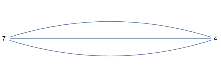
The result may contain self-loops. The smallest topological equivalent of a cycle graph is a single vertex with a self-loop.
IGSmoothen[CycleGraph[10]]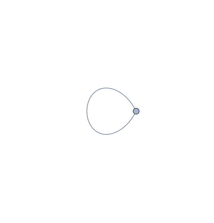
The result may also contain multi-edges.

If the input is directed, only those vertices are smoothed which have one incoming and one outgoing edge.
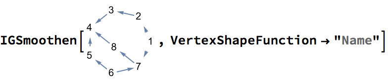
Use DirectedEdges -> False to treat the input graph
as undirected.
The result is always a weighted graph. When contracting edges, their weights are added up. If the input graph was not weighted, all of its edge weights are considered to be 1. Thus, the graph distance of any two vertices in the result is always the same as it was in the input graph.
g = IGGiantComponent@RandomGraph[{100, 100}]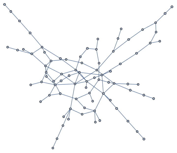
tm = IGSmoothen[g]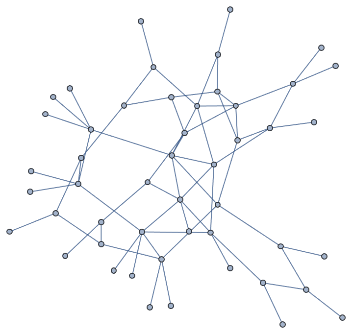
IGEdgeWeightedQ[tm]True
IGDistanceMatrix[g, VertexList[tm], VertexList[tm]] ==
 IGDistanceMatrix[tm]
True
The result does not contain any degree-2 vertices, except possibly isolated vertices with self-loops.
Union@VertexDegree[tm]{1, 3, 4, 5, 6}
The vertex coordinates, as well as any other graph properties are discarded.
g = IGMeshGraph@IGLatticeMesh["Hexagonal", {3, 3}]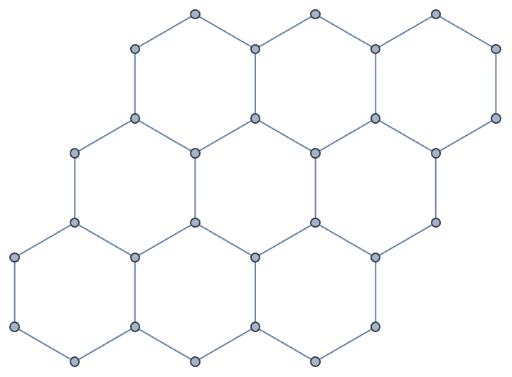
IGSmoothen[g]
Vertex coordinates can be transferred to the new graph as follows:
IGSmoothen[g,
 VertexCoordinates -> {v_ :>
    PropertyValue[{g, v}, VertexCoordinates]}]
An alternative and faster method uses IGVertexMap and
IGVertexAssociate:
IGSmoothen[g] //
 IGVertexMap[IGVertexAssociate[GraphEmbedding][g],
  VertexCoordinates -> VertexList]
Create a tree in which every non-leaf node has a degree of at least 3.
IGSmoothen[IGTreeGame[100], GraphLayout -> "RadialEmbedding"]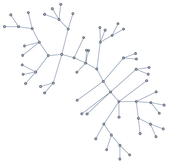
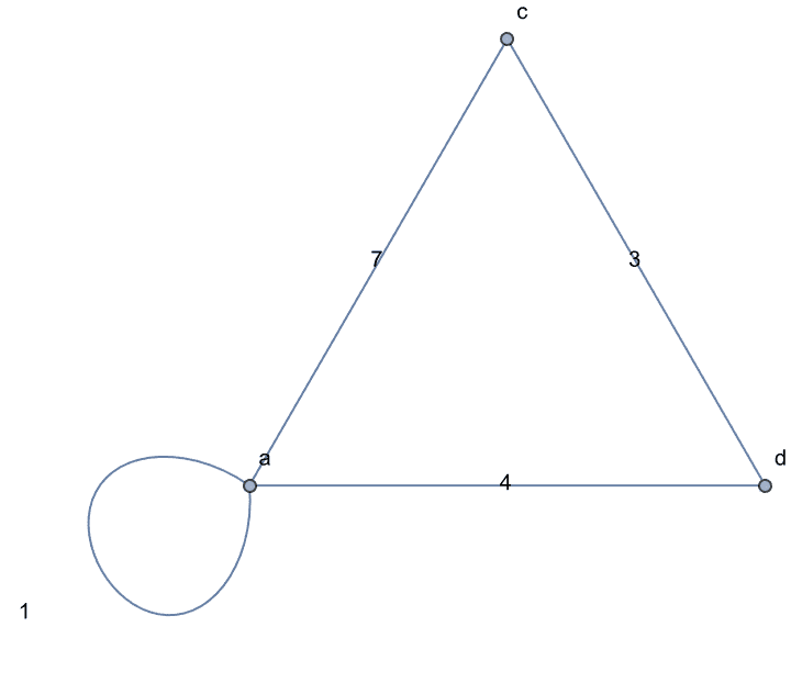
Let us compute the effective resistance of a resistor network by repeated smoothing (merger of resistors in series) and simplification (merger of resistors in parallel). Resistances are stored as edge weights. A zero-resistance input and output terminal is added to prevent the premature smoothing of these points.
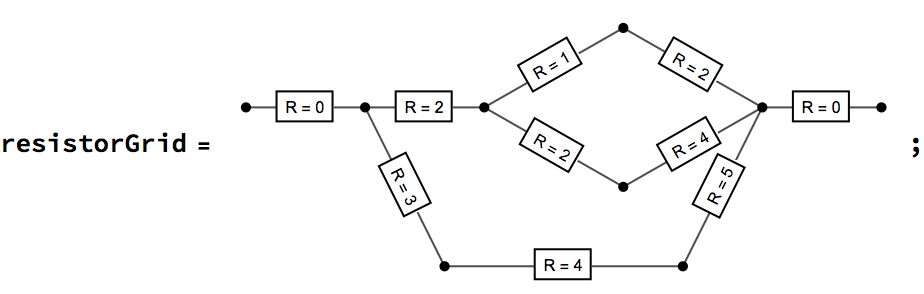
Merge resistors in series …
reducedGrid = IGSmoothen[resistorGrid]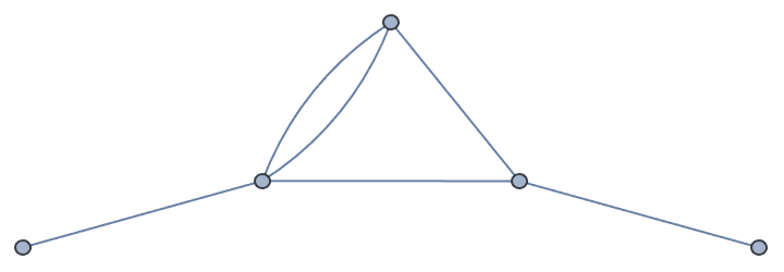
… then merge resistors in parallel and check the resulting edge weights.
reducedGrid =
 IGWeightedSimpleGraph[reducedGrid, 1/Total[1/{##}] &,
  EdgeLabels -> "EdgeWeight"]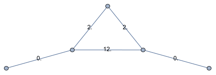
Repeat until a single resistor remains.
reducedGrid = IGSmoothen[reducedGrid]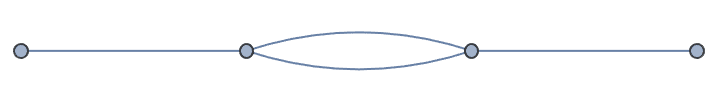
reducedGrid =
 IGWeightedSimpleGraph[reducedGrid, 1/Total[1/{##}] &,
EdgeLabels -> "EdgeWeight"]![]()
reducedGrid = IGSmoothen[reducedGrid, EdgeLabels -> "EdgeWeight"]![]()
IGEdgeProp[EdgeWeight][reducedGrid]{3.}
Centralities are various measures that quantify the “importance” of vertices or edges in graphs.
?IGBetweenness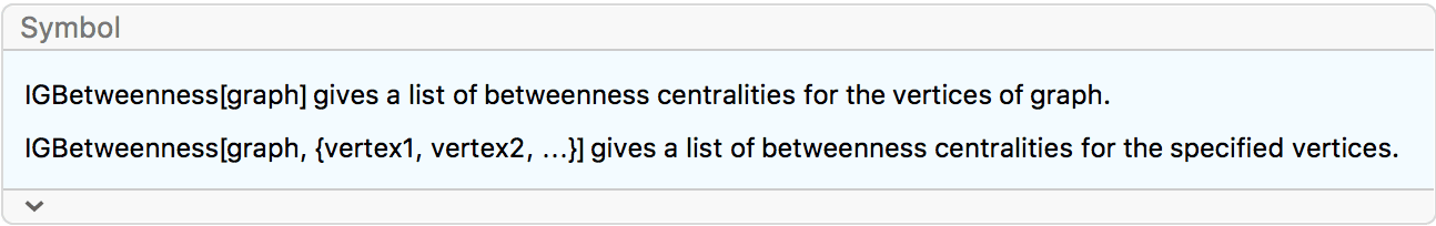
?IGBetweennessCutoff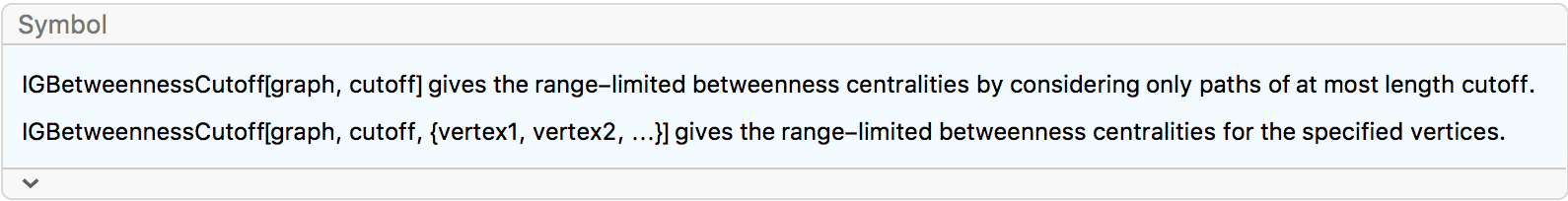
?IGEdgeBetweenness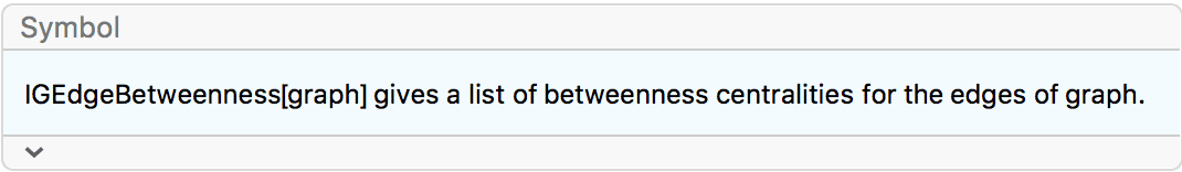
?IGEdgeBetweennessCutoff
The betweenness of a vertex or edge is, roughly speaking, the number of shortest paths passing through it. More formally, the betweenness of vertex \(i\) is \(b_i=\sum _{i\neq s\neq t} \frac{g_{st}^{(i)}}{g_{st}}\), where \(g_{st}\) is the total number of shortest paths (geodesics) between vertices \(s\) and \(t\), and \(g_{st}^{(i)}\) is the number of shortest paths between vertices \(s\) and \(t\) that pass through \(i\).
Weighted graphs and multigraphs are supported by all betweenness functions in IGraph/M.
Note that as of Mathematica 13.0, the built-in
BetweennessCentrality function ignores edge weights and
multi-edges, which causes it to yield different results from
IGBetweenness.
Available options:
Normalized -> True will compute the normalized
betweenness by dividing the result by the number of (ordered or
unordered) vertex pairs used in the shortest path calculation. Thus the
normalization factor is \((V-1) (V-2)\)
for directed graphs and \(\frac{1}{2} (V-1)
(V-2)\) for undirected graphs. The normalized value lies between
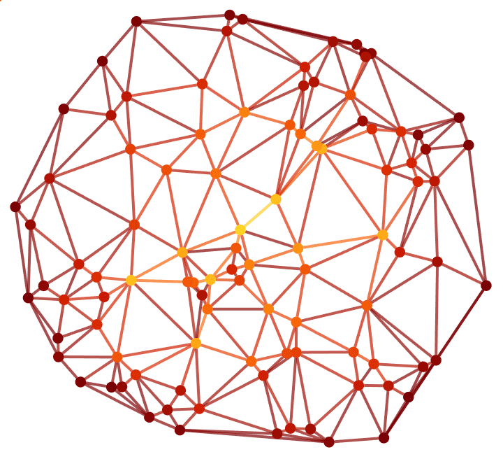
0 and 1.Visualize the vertex and edge betweenness of a weighted geometrical graph, where weights represent Euclidean distances.
pts = RandomPoint[Disk[], 100];
IGMeshGraph[
  DelaunayMesh[pts],
  EdgeStyle -> Thick, VertexStyle -> EdgeForm[None]
  ] //
 IGVertexMap[
   ColorData["SolarColors"],
   VertexStyle -> Rescale@*IGBetweenness
   ]/*
  IGEdgeMap[
   ColorData["SolarColors"],
   EdgeStyle -> Rescale@*IGEdgeBetweenness
   ]
Compute the betweenness of a subset of vertices.
g = ExampleData[{"NetworkGraph", "DolphinSocialNetwork"}];Take[VertexList[g], 5]{"Beak", "Beescratch", "Bumper", "CCL", "Cross"}
IGBetweenness[g, %]{34.9212, 390.384, 16.6032, 4.34405, 0.}
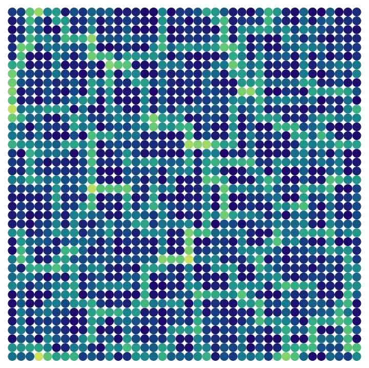
Visualize the betweenness of a periodic grid with slightly randomized edge weights.
n = 40;
IGSquareLattice[{n, n},
  "Periodic" -> True,
  VertexCoordinates -> Tuples[Range[n], {2}],
  EdgeWeight -> {_ :> RandomReal[{.99, 1.01}]},
  GraphStyle -> "BasicBlack",
  EdgeShapeFunction -> None,
  VertexSize -> 1
  ] // IGVertexMap[
  ColorData["BlueGreenYellow"],
  VertexStyle -> Rescale@*IGBetweenness
  ]
Betweenness computation involves comparing the lengths of paths, and deciding which specific path is the shortest, and which paths have equal lengths. When non-integer edge weights are used, the path length computation is subject to roundoff errors, which may cause the path length comparison to fail. igraph mitigates this by comparing the lengths using tolerances, however, there is still a small risk that roundoff errors may affect the result. To avoid this potential problem entirely, use integer weights. For example, if the weights are rational, multiply them by the least common multiple of their denominators.
?IGCloseness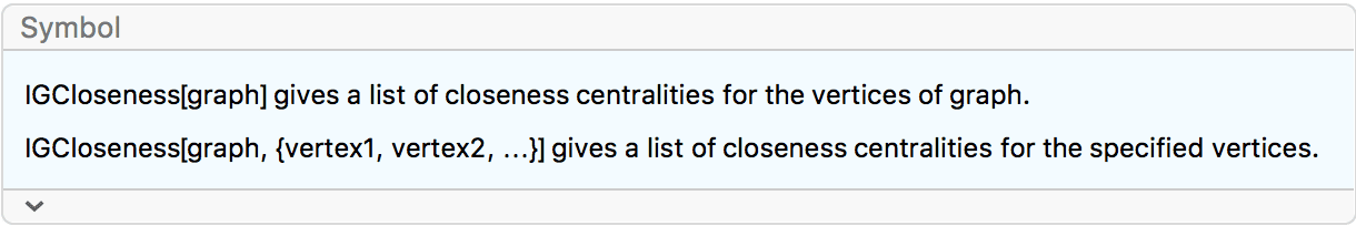
?IGClosenessCutoff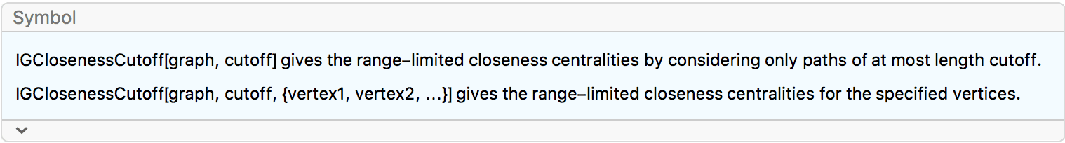
?IGNeighborhoodCloseness
The normalized closeness centrality of a vertex is the inverse average shortest path length to other vertices.
Weighted graphs are supported.
Available options:
Normalized -> False will compute the non-normalized
closeness, i.e. the inverse of the sum of shortest path lengths to all
other vertices.There is no standard definition of closeness centrality for
disconnected graphs. When the graph is disconnected, IGraph/M will only
consider the distances to reachable vertices. In the undirected case,
this effectively computes the closeness separately for each connected
component. Use IGNeighborhoodCloseness to obtain both the
closeness values, as well as how many vertices were reachable from each
vertex. This information allows for computing various generalizations of
closeness centrality for disconnected graphs.
Visualize the closeness of nodes in a weighted geometrical graph where weights correspond to Euclidean distances.
pts = RandomPoint[Polygon@CirclePoints[3], 75];
IGVertexMap[
 ColorData["Rainbow"],
 VertexStyle -> Rescale@*IGCloseness,
 IGMeshGraph[DelaunayMesh[pts], GraphStyle -> "BasicBlack"]
 ]
For isolated vertices, Indeterminate is returned.
IGCloseness@IGShorthand["1,2-3"]{Indeterminate, 1., 1.}
?IGHarmonicCentrality
?IGHarmonicCentralityCutoff
The harmonic centrality of a vertex is the average inverse shortest path length to all other vertices. The inverse shortest path length to unreachable vertices is considered to be zero.
Available options:
Normalized -> False computes the non-normalized
harmonic centrality, i.e. the sum of inverse shortest path length to all
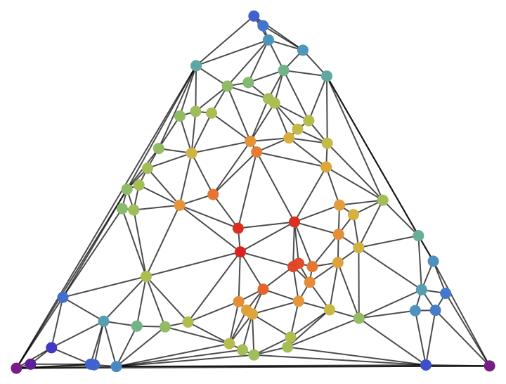
other vertices.RandomGraph[{30, 40}, VertexSize -> Large] //
IGVertexMap[ColorData["Rainbow"],
VertexStyle -> IGHarmonicCentrality/*Rescale]
?IGPageRank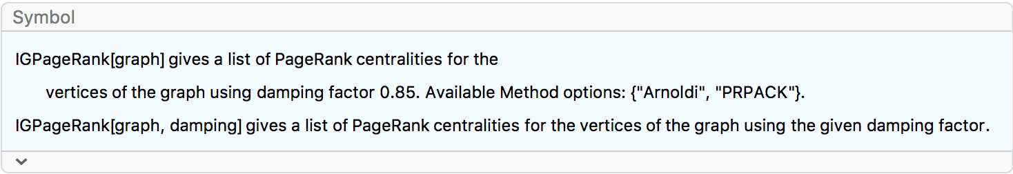
?IGPersonalizedPageRank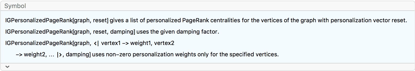
The PageRank centrality of a vertex is the fraction of time a random walker would spend on that vertex. The walker jumps from vertex to vertex randomly, following outward edges with probabilities proportional to their weights. Additionally, after each step, with a probability \(1-d\) the walk is restarted from a random vertex. \(d\) is called the damping factor. If the walker is stuck in a sink vertex (i.e. a vertex with no outgoing edges), the walk is also restarted.
In the standard version of PageRank, when the walk is restarted, the
starting vertex is chosen uniformly. In the personalized version, it is
chosen with probabilities proportional to the values in the
reset parameter.
Weighted graphs and multigraphs are supported, and self-loops are taken into consideration.
Note that as of Mathematica 13.0, the built-in
PageRankCentrality function ignores self-loops.
The default damping factor is 0.85.
The following Method options are available:
"Arnoldi" uses ARPACK, and solves PageRank as an
eigenvalue problem.
"PRPACK" uses PRPACK and uses the
algebraic method. It is the default method, and usually much faster than
"Arnoldi".
Plot the logarithmic histogram of PageRank scores of the network of webpage in the nd.edu domain.
ndWeb = ExampleData[{"NetworkGraph", "WorldWideWeb"}];Histogram[IGPageRank[ndWeb], "Log", {"Log", "PDF"},
Frame -> True, FrameLabel -> {"PageRank", "PDF"}]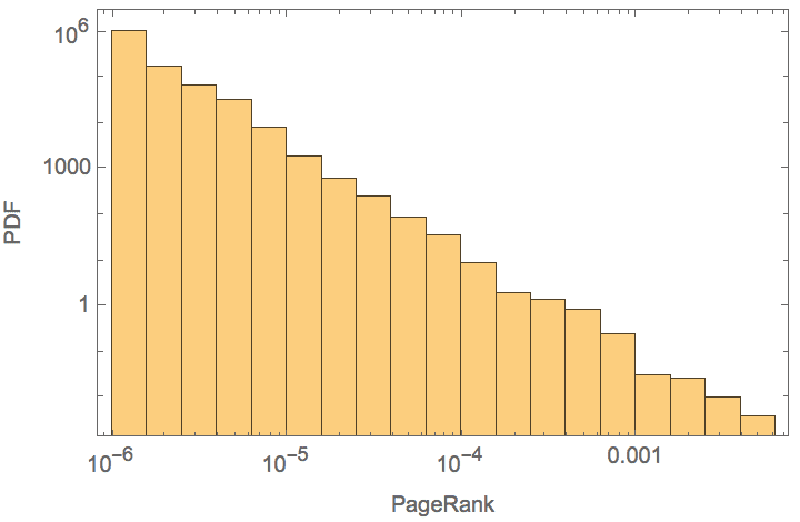
The personalization weights may be given as a vector of the same length as the vertex list …
g = RandomGraph[{10, 20}, DirectedEdges -> True];
IGPersonalizedPageRank[g, RandomReal[1, VertexCount[g]]]{0.0433579, 0.129471, 0.23356, 0.113496, 0.000101892, 0.12872, \ 0.260584, 0.024101, 0.0324582, 0.0341504}
… or as an association from vertex names to weights, in which case the weight of non-included vertices is taken to be zero.
IGPersonalizedPageRank[g, <|1 -> 1.5, 3 -> 0.5|>]{0.297935, 0.0717967, 0.168933, 0.290878, 0., 0.0376334, 0.132824, \ 0., 0., 0.}
Personalize PageRank by always restarting the walk from one of two vertices (29 or 74) on a grid graph:
g = IGSquareLattice[{10, 10}, VertexSize -> Large];g // IGVertexMap[ColorData["Rainbow"],
VertexStyle -> (IGPersonalizedPageRank[#, <|29 -> 1, 74 -> 1|>,
0.99] &/*Rescale)]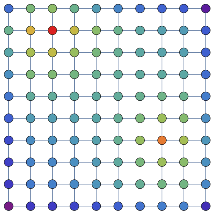
?IGLinkRank
?IGPersonalizedLinkRank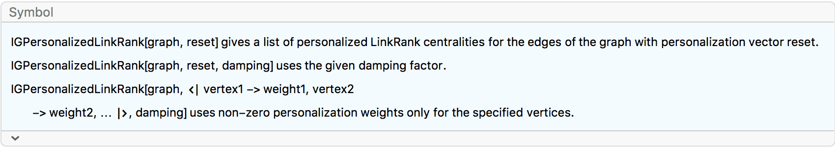
LinkRank is the equivalent of PageRank for edges. The LinkRank of an edge is the relative frequency of traversing that edge by a random walker. For a detailed description of the random walk process, see the PageRank section.
The LinkRank of edges can be computed from the PageRank by simply dividing the PageRank of each vertex between its outgoing edges, proportionally with their edge weights. The LinkRank scores of the out-edges of a vertex add up to the PageRank of that vertex. The LinkRank scores of all edges in the graph add up to 1.
Weighted graphs and multigraphs are supported, and self-loops are taken into consideration.
The available Method options are the same as for
IGPageRank.
Visualize both the LinkRank and PageRank of a random directed graph.
maxNorm = #/Max[#] &;

g = RandomGraph[{15, 30}, DirectedEdges -> True, EdgeStyle -> Thick,
   VertexSize -> Large, GraphStyle -> "BasicBlack"];

g // IGEdgeMap[ColorData["Rainbow"],
   EdgeStyle -> IGLinkRank/*maxNorm] //
 IGVertexMap[ColorData["Rainbow"], VertexStyle -> IGPageRank/*maxNorm]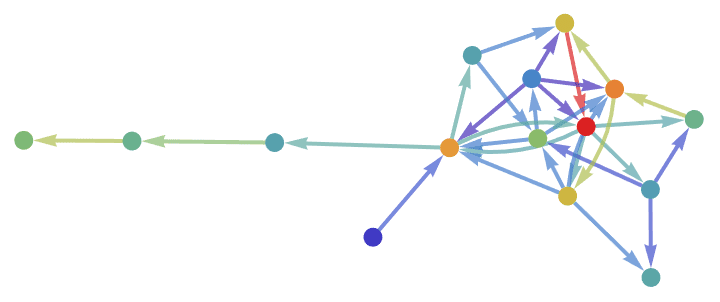
Visualize the personalized version of LinkRank and PageRank, always starting the random walk from vertex 1.
pers = <|1 -> 1|>;
Graph[g, VertexLabels -> "Name"] //
  IGEdgeMap[ColorData["Rainbow"],
   EdgeStyle -> (IGPersonalizedLinkRank[#, pers] &)/*maxNorm] //
 IGVertexMap[ColorData["Rainbow"],
  VertexStyle -> (IGPersonalizedPageRank[#, pers] &)/*maxNorm]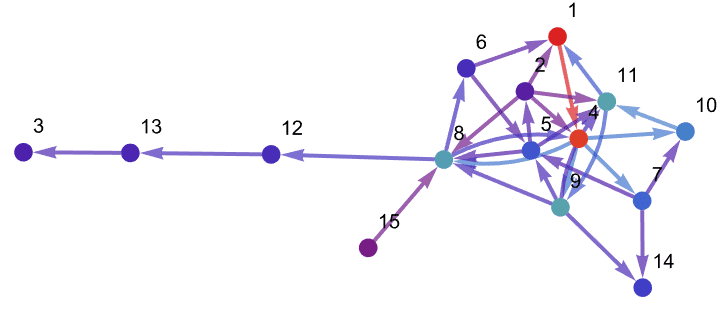
?IGEigenvectorCentrality
Eigenvector centrality is based on the idea that the importance (centrality) of a vertex should be affected not only by how many other vertices point to it, but also by the importance of its neighbours. The eigenvector centrality of a vertex is proportional to the sum of centralities of its neighbours. Mathematically, the eigenvector centrality is the leading eigenvector of the adjacency matrix.
Eigenvector centrality is meaningful for connected graphs only. Disconnected graphs should be decomposed into their components, and the eigenvector centrality computed separately for each. The vertex centrality scores will be comparable only within components, not between separate components.
In undirected graphs, the diagonal of the adjacency matrix is assumed to contain twice the number of self-loops on each vertex. This makes the undirected result consistent with the directed one when each undirected edge is replaced by reciprocal directed ones.
For directed graphs, the left eigenvector of the adjacency matrix is calculated. In other words, the centrality of a vertex is proportional to the sum of centralities of vertices pointing to it.
Weighted and directed graphs are supported.
The available options are:
Normaized -> True will scale the result so that
the maximum centrality is 1. The default is True.
DirectedEdges -> False ignores edge
directions.
?IGHubScore
?IGAuthorityScore
Weighted graphs are supported.
The available options are:
Normalized -> True scales the result so that the
maximum centrality is 1. The default is True.?IGConstraintScore
Weighted graphs are supported.
?IG*Centralization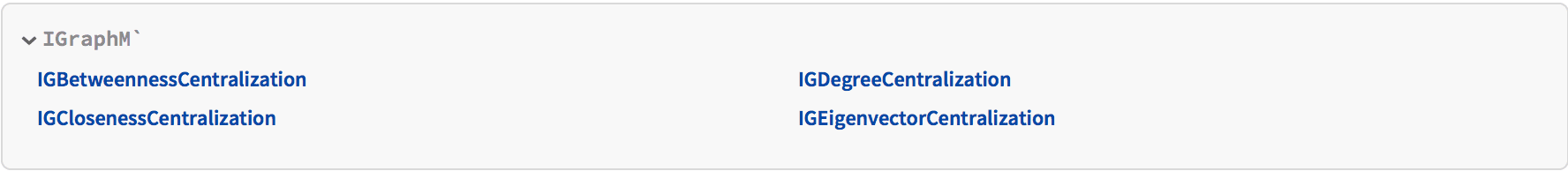
Centralization is computed from centrality values in a way
equivalent to Total[Max[centralities] - centralities]. With
the (default) option Normalized -> True, the result is
normalized by dividing by the highest possible centralization score of
any graph of the same directedness on the same number of vertices.
g = IGBarabasiAlbertGame[100, 2, DirectedEdges -> False];IGBetweennessCentralization[g]0.194343
IGClosenessCentralization[g]0.275726
IGDegreeCentralization[g, SelfLoops -> False]0.144919
IGEigenvectorCentralization[g]0.820631
For most centrality types, the highest centralization is achieved by
the StarGraph.
IGBetweennessCentralization@StarGraph[5]1.
In the case of the degree centralization, the highest possible
centralization score depends on whether self-loops are allowed. This is
controlled by the SelfLoops option of
IGDegreeCentralization. The default is
SelfLoops -> True.
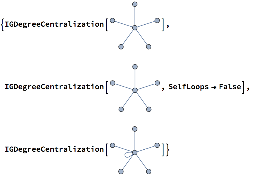
{0.666667, 1., 1.}
?IGDirectedAcyclicGraphQ
IGDirectedAcyclicGraphQ tests if a graph is directed and
has no directed cycles.
IGDirectedAcyclicGraphQ /@ {IGShorthand["1->2->3->1"],
IGShorthand["1->2->3<-1"]}{False, True}
IGDirectedAcyclicGraphQ returns True for
graphs with no edges.
IGDirectedAcyclicGraphQ[IGEmptyGraph[3]]True
?IGTopologicalOrdering
IGTopologicalOrdering is to the built-in
TopologicalSort as Ordering is to
Sort: it returns the permutation which sorts vertices in
topological order. When vertices are ordered topologically, all directed
edges point from earlier vertices to later ones.
Graphs must be acyclic for topological sorting to be possible.
IGDirectedAcyclicGraphQ[g]True
p = IGTopologicalOrdering[g]{5, 8, 9, 4, 6, 1, 2, 3, 10, 7}
VertexList[g][[p]]{"E", "H", "I", "D", "F", "A", "B", "C", "J", "G"}
If the vertices are laid out from left to right in topological order, all edges will point from left to right.
curvedEdge[offset_][{a_, ___, b_}, ___] :=
 Arrow@BezierCurve[{a, (a + b)/2 + offset Reverse[b - a], b}]
Graph[g,
  EdgeShapeFunction -> curvedEdge[2/3] (*
  in M12.0 or later simply use {{"CurvedEdge",
  "Curvature"->1.5}} *)
  ] // IGVertexMap[{#, 0} &,
  VertexCoordinates -> IGTopologicalOrdering/*Ordering]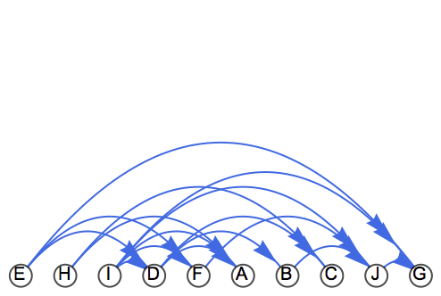
When the graph contains cycles, $Failed is returned.
IGTopologicalOrdering[IGShorthand["1->2->3->4->5, 5->3, 5->6"]]![]()
![]()
$Failed
?IGFeedbackArcSet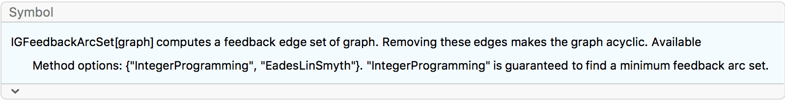
IGFeedbackArcSet[] returns a set of directed edges (also
called arcs) the removal of which makes the graph acyclic.
With Method -> "IntegerProgramming", it finds an
exact minimal feedback arc set through integer programming using the
triangle inequality formulation. With
Method -> "EadesLinSmyth", it finds a feedback arc set
(not necessarily minimal) using the fast “GR” heuristic of Eades, Lin
and Smyth (1993).
The following directed graph is not acyclic.
g = RandomGraph[{10, 20}, DirectedEdges -> True,
  VertexLabels -> "Name"]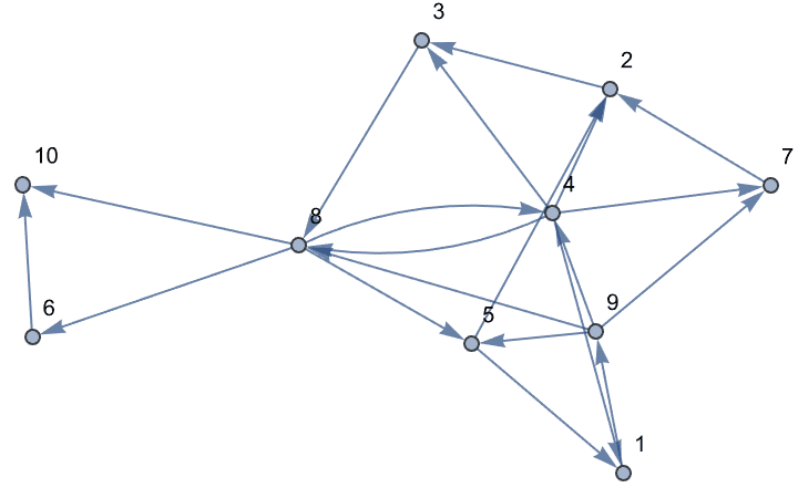
{AcyclicGraphQ[%], IGDirectedAcyclicGraphQ[%]}{False, False}
Find a set of edges whose removal breaks all cycles.
IGFeedbackArcSet[g]{1 \[DirectedEdge] 9, 3 \[DirectedEdge] 8, 4 \[DirectedEdge] 8}
ag = EdgeDelete[g, %]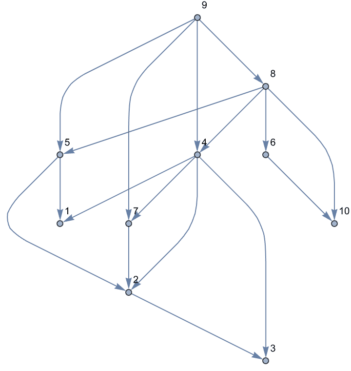
IGDirectedAcyclicGraphQ[ag]True
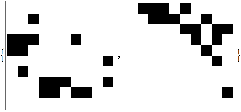
Vertices of a directed acyclic graph can be sorted topologically.
IGTopologicalOrdering returns a permutation that sorts them
this way, and thus makes the graph’s adjacency matrix upper
triangular.
perm = IGTopologicalOrdering[ag]{9, 8, 4, 5, 6, 7, 1, 10, 2, 3}
With[{am = AdjacencyMatrix[ag]},
 ArrayPlot /@ {am, am[[perm, perm]]}
 ]
Chordal graphs are graphs that do not contain induced cycles with more than three vertices.
?IGChordalQ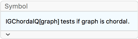
A graph is chordal if each of its cycles of four or more nodes has a chord, i.e. an edge joining two non-adjacent vertices in the cycle. Equivalently, all chordless cycles in a chordal graph have at most 3 vertices.
Chordal graphs are also called rigid circuit graphs or triangulated graphs.
Grid graphs are not chordal because they have chordless 4 cycles.
g = GridGraph[{2, 3}, VertexLabels -> "Name"]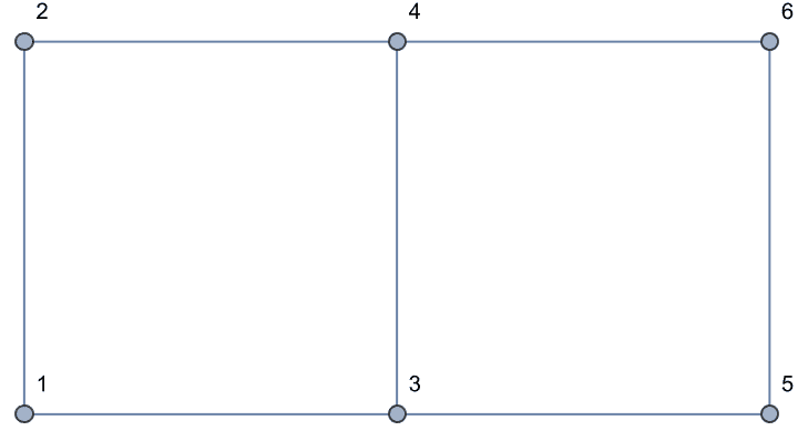
IGChordalQ[g]False
Adding chords to the 4 cycles makes them chordal.
EdgeAdd[g, {1 <-> 4, 4 <-> 5}]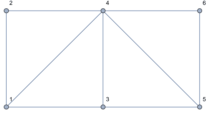
IGChordalQ[%]True
?IGChordalCompletion
IGChordalCompletion computes a set of edges that, when
added to a graph, make it chordal. The edge set returned is not usually
minimal, i.e. some of the edges may not be necessary to create a chordal
graph.
g = CycleGraph[5]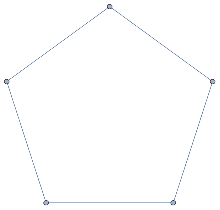
completion = IGChordalCompletion[g];
HighlightGraph[EdgeAdd[g, completion], completion]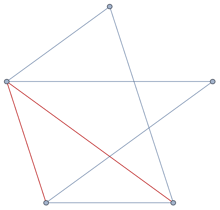
?IGMaximumCardinalitySearch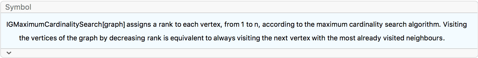
The maximum cardinality search algorithm visits the vertices of the
graph in such an order so that every time the vertex with the most
already visited neighbours is visited next. Ties are broken arbitrarily.
Then vertices are assigned ranks \(\alpha\) in decreasing order from the
vertex count of the graph to 1. IGMaximumCardinalitySearch
returns these ranks.
The visiting order is animated below:
ranks = AssociationThread[VertexList[g],
IGMaximumCardinalitySearch[g]]<|1 -> 10, 2 -> 3, 3 -> 8, 4 -> 6, 5 -> 7, 6 -> 2, 7 -> 1, 8 -> 5, 9 -> 4, 10 -> 9|>
verts = Keys@Reverse@Sort[ranks]
Table[
  HighlightGraph[
   Graph[g, VertexLabels -> "Name"],
   Take[verts, i]
   ],
  {i, VertexCount[g]}
] // ListAnimate{1, 10, 3, 5, 4, 8, 9, 2, 6, 7}
The rank \(\alpha\) is useful for deciding the chordality of a graph. A graph is chordal if and only if any two neighbors of a vertex which are higher in rank than it are connected to each other.
Label the vertices of a graph with their ranks.
g = IGShorthand["a-b-c-d-a-e-f-g-h-e-g"];
IGVertexMap[Row[{#1, ": ", #2}] &,
 VertexLabels -> {VertexList, IGMaximumCardinalitySearch}, g]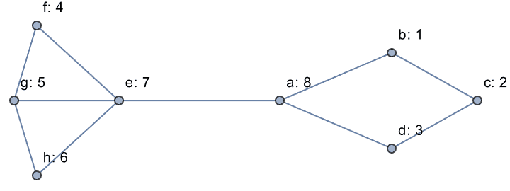
Notice that vertex b has two higher-rank neighbours that
are not connected to each other. This graph is not chordal. Use
IGChordalCompletion to determine which edges to add to it
to make it chordal.
IGChordalCompletion[g]{"c" <-> "a"}
?IG*ClusteringCoefficient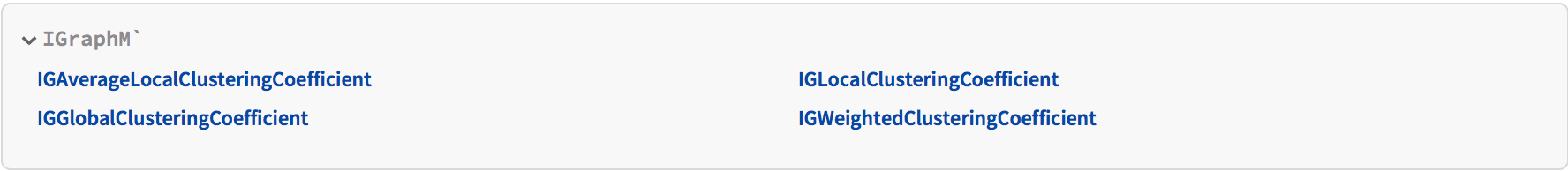
Clustering coefficients are measures of the degree to which vertices in a graph tend to cluster together. They are also referred to as transitivity, as they measure how often two vertices that are connected through a third one are also directly connected.
All clustering coefficient calculations in IGraph/M ignore edge directions.
?IGGlobalClusteringCoefficient
The clustering coefficient of an undirected graph is defined as
\[C=\frac{\text{number of closed ordered triplets}}{\text{number of connected ordered triplets}}\]
The available options are:
"ExcludeIsolates" -> True will cause
Indeterminate to be returned if the graph has no connected
triplets. With the default "ExcludeIsolates" -> False,
0 is returned.The following graph has 10 connected ordered triplets, namely {3, 1,
2}, {2, 1, 3}, {1, 2, 3}, {3, 2, 1}, {2, 3, 1}, {2, 3, 4}, {1, 3, 4},
{1, 3, 2}, {4, 3, 2}, {4, 3, 1}. Out of these, only 6 are closed: {1, 3,
2}, {1, 2, 3}, {2, 1, 3}, {2, 3, 1}, {3, 2, 1}, {3, 1, 2}. Thus the
clustering coefficient is 6/10 = 0.6.
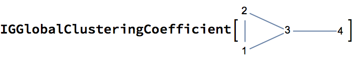
0.6
?IGLocalClusteringCoefficient
The local clustering coefficient of a vertex is defined as
\[C=\frac{\text{number of connected pairs of neighbours}}{\text{total number of pairs of neighbours}}\]
The available options are:
"ExcludeIsolates" -> True will cause
Indeterminate to be returned for degree 0 and degree 1
vertices. With the default "ExcludeIsolates" -> False,
0 is returned.The the following graph, vertex 4 has two neighbours which are
disconnected, making its local clustering zero. However, vertex 5 has
only one neighbour, thus computing the local clustering for it arguably
does not make sense. Setting "ExcludeIsolates" -> True
serves to distinguish these two cases by returning
Indeterminate for vertex 5.
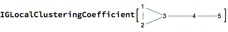
{1., 1., 0.333333, 0., 0.}

{1., 1., 0.333333, 0., Indeterminate}
?IGAverageLocalClusteringCoefficient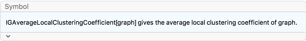
The available options are:
"ExcludeIsolates" -> True will cause degree 0 and
degree 1 vertices to be excluded from the calculation.With "ExcludeIsolates" -> True, the local clustering
coefficient of vertex 4 will be excluded from the calculation of the
average.
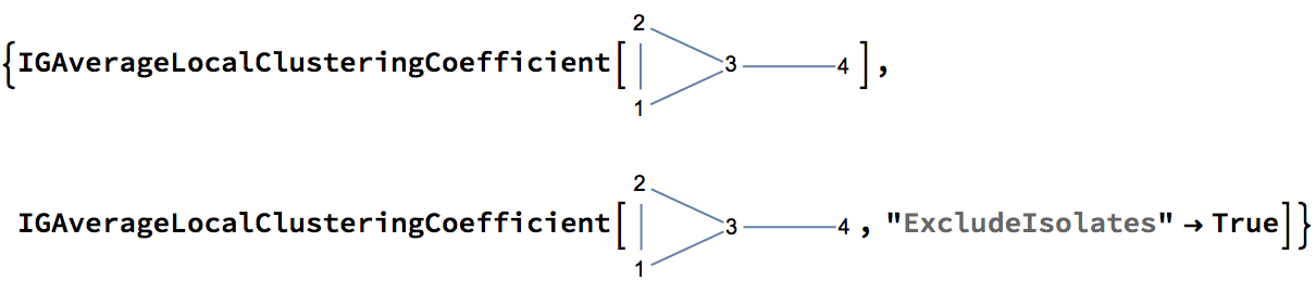
{0.583333, 0.777778}
When the graph has no vertices with degree of at least 2, and
"ExcludeIsolates" -> True is set, the result will be
Indeterminate.
![]()
Indeterminate
?IGWeightedClusteringCoefficient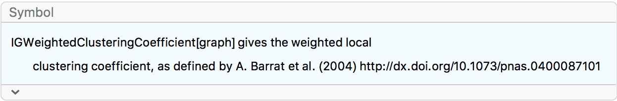
IGWeightedClusteringCoefficient computes the
weighted local clustering coefficient. This function expects a
weighted graph as input.
The available options are:
"ExcludeIsolates" -> True will cause
Indeterminate to be returned for degree 0 and degree 1
vertices. With the default "ExcludeIsolates" -> False,
0 is returned.?IGAverageNeighborDegree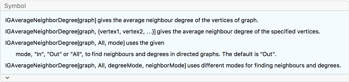
IGAverageNeighborDegree computes the average of the
degrees of each vertex’s neighbours. In weighted graphs, a weighted
average is used:
\[k_{\text{nn},u}=\frac{1}{s_u}\sum _v w_{uv}k_v\]
\(k_{\text{nn},u}\) denotes the average neighbour degree of vertex \(u\), \(k_v\) is the degree of vertex \(v\), \(w_{uv}\) is the weighted adjacency matrix, and \(s_u=\sum _vw_{uv}\) is the strength of vertex \(u\).
IGAverageNeighborDegree is similar to
MeanNeighborDegree, with a few differences: it can compute
the measure for only a subset of vertices, the interpretation of degrees
and neighbours can be controlled independently in directed graphs, and
for vertices which have no neighbours it returns
Indeterminate instead of 0.
Average neighbour degree in a star graph:
IGAverageNeighborDegree[StarGraph[4]]{1., 3., 3., 3.}
Compute the result only for vertices 1 and 3:
IGAverageNeighborDegree[StarGraph[4], {1, 3}]{1., 3.}
All computes the result for all vertices (the
default):
IGAverageNeighborDegree[StarGraph[4], All]{1., 3., 3., 3.}
When a vertex has no neighbours, Indeterminate is
returned:
IGAverageNeighborDegree[IGShorthand["1,2-3"]]{Indeterminate, 1., 1.}
In directed graphs, the out-degrees of out-neighbours are considered by default.
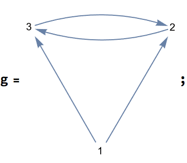
IGAverageNeighborDegree[g]{1., 1., 1.}
Use in-degrees of in-neighbours instead:
IGAverageNeighborDegree[g, All, "In"]{Indeterminate, 1., 1.}
Use the in-degrees of all neighbours:
IGAverageNeighborDegree[g, All, "In", "All"]{2., 1.33333, 1.33333}
Compute a weighted neighbour degree average. The weights used in averaging are taken from the edge weights:
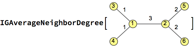
{2.2, 1.85714, 3., 3., 3., 3.}
?IGAverageDegreeConnectivity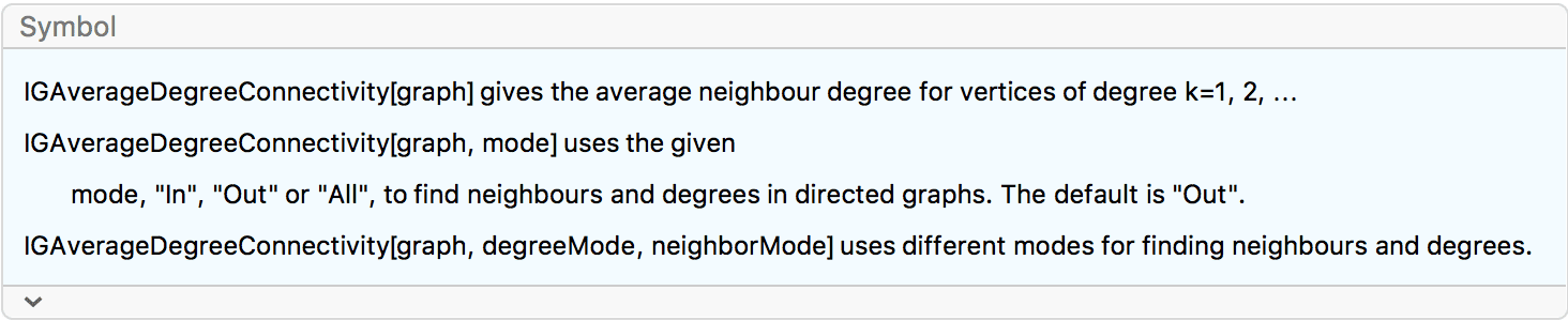
IGAverageDegreeConnectivity computes the average
neighbour degree as a function of the vertex degree. The \(i\)th element of the result is the average
of the IGAverageNeighborDegree result for all vertices of
degree \(i\).
g = RandomGraph[{30, 50}];IGAverageDegreeConnectivity[g]{3., 3.92857, 3.44444, 4.21429, 4.46667, 4.33333, Indeterminate, \ 4.125}
An equivalent implementation of
IGAverageDegreeConnectivity is:
Transpose[{VertexDegree[g], IGAverageNeighborDegree[g]}] //
  GroupBy[#, First -> Last, Mean] & //
Lookup[#, Range@Max@VertexDegree[g], Indeterminate] &{3., 3.92857, 3.44444, 4.21429, 4.46667, 4.33333, Indeterminate, \ 4.125}
Compute the average degree connectivity curve for a scale free network:
ListPlot[
 IGAverageDegreeConnectivity@IGStaticPowerLawGame[1000, 2000, 2],
 FrameLabel -> {"degree", "average neighbour degree"},
 PlotTheme -> "Detailed"
 ]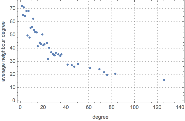
The length of a path between two vertices is the number of edges the path consists of. Functions that use edge weights consider the path length to be the sum of edge weights along the path.
?IGDistanceMatrix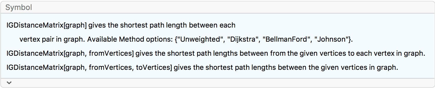
IGDistanceMatrix takes the following Method
options:
Automatic selects a method automatically. As of
IGraph/M 0.5, "Unweighted" is selected for unweighted
graphs, "Dijkstra" for weighted graphs with only positive
weights, and "Johnson" otherwise.
"Unweighted" ignores weights
"Dijkstra" uses Dijkstra’s algorithm. All weights
must be non-negative.
"BellmanFord" uses the Bellman–Ford algorithm.
Negative weights are supported but all cycles must have a non-negative
total weight.
"Johnson" uses the Johnson algorithm. Negative
weights are supported but all cycles must have a non-negative total
weight.
The igraph C core may override explicit method settings when
appropriate. For example, if the graph is not weighted, it always uses
"Unweighted".
?IGDistanceCounts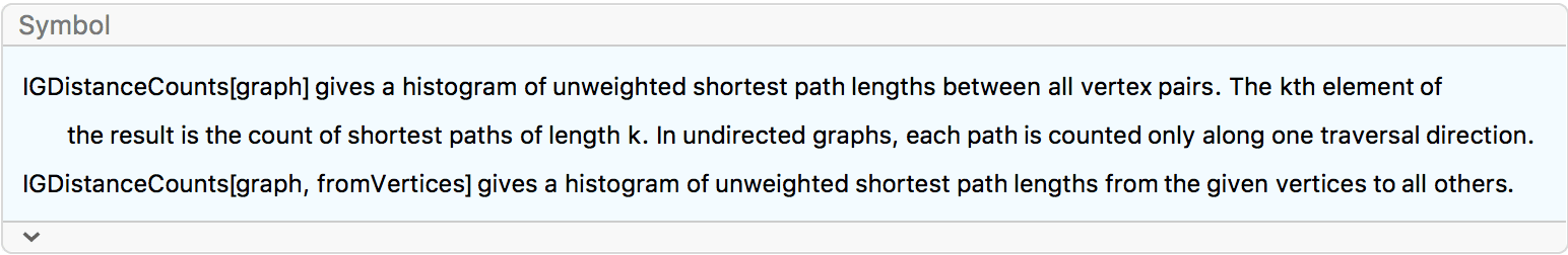
IGDistanceCounts[graph] counts all-pair
unweighted shortest path lengths in the graph.
![]() counts unweighted shortest path lengths for paths starting at the given
vertices.
counts unweighted shortest path lengths for paths starting at the given
vertices.
For weighted path lengths, or to restrict the computation to both
certain start and end vertex sets, use
IGDistanceHistogram[].
Compute how the shortest path length distribution changes as we
rewire a grid graph k times.
Table[
 ListPlot[
  Normalize[IGDistanceCounts@IGRewire[GridGraph[{50, 50}], k],
   Total],
  Joined -> True, Filling -> Bottom,
  PlotLabel -> StringTemplate["rewiring steps: ``"][k]
  ],
 {k, {0, 5, 10, 20, 50, 100}}
 ]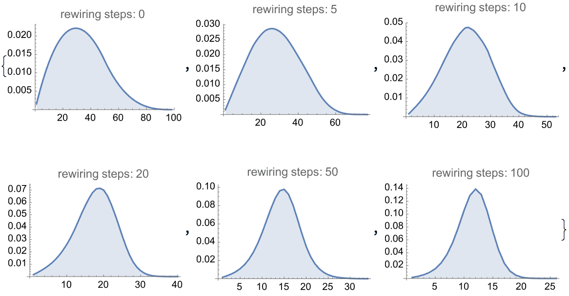
?IGNeighborhoodSize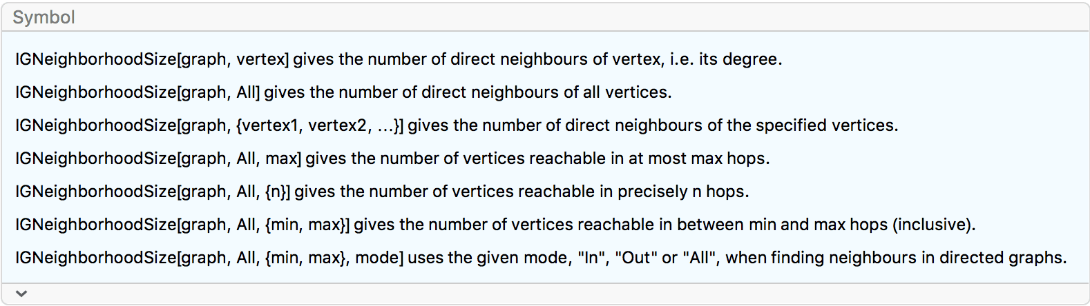
IGNeighborhoodSize returns the number of vertices
reachable within a certain distance range from a given vertex, or from
multiple given vertices.
Scale vertices proportionally to the number of their second order neighbours:
g = IGBarabasiAlbertGame[50, 2, DirectedEdges -> False];
IGVertexMap[# &,
 VertexSize -> (Rescale@IGNeighborhoodSize[#, All, {2}] &), g]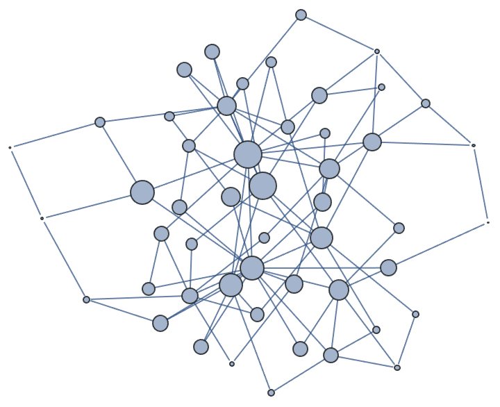
?IGDistanceHistogram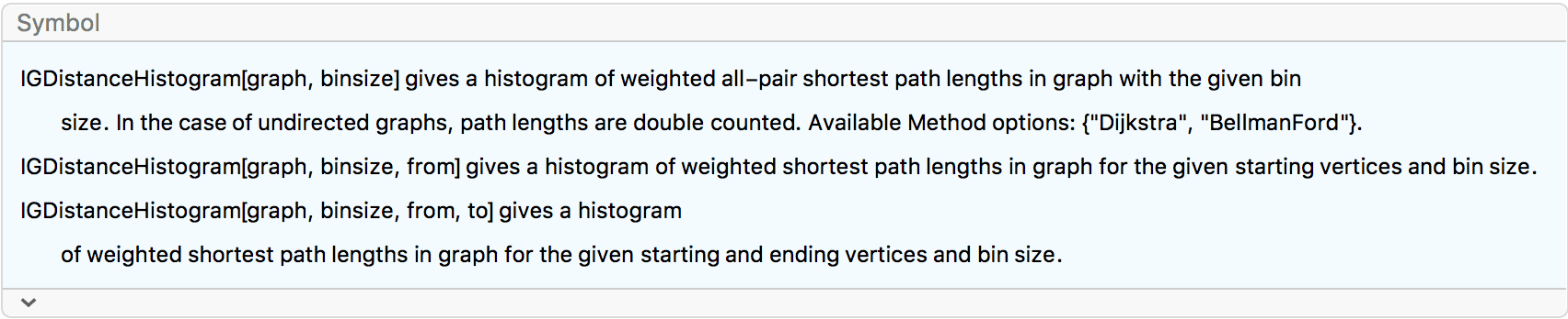
IGDistanceHistogram[] computes the weighted shortest
path length histogram between the specified start and end vertex sets.
The start and end vertex sets do not need to be the same. Note that if
the graph is undirected, path lengths between s and
t will be double counted (from s -> t and
t -> s) if s and t appear both
in the starting and ending vertex sets.
IGDistanceHistogram[] is useful when the result of
IGDistanceMatrix[] (or GraphDistanceMatrix[])
does not fit in memory.
?IGAveragePathLength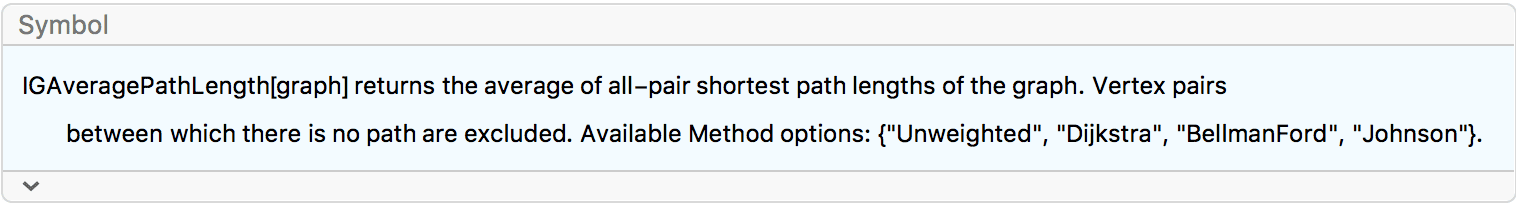
IGAveragePathLength computes the average pairwise
distances between vertices.
Available options:
Method can take the values
"Unweighted", "Dijkstra",
"BellmanFord", "Johnson" and
Automatic. Automatic uses
"Unweighted" if no edge weights are present,
"Dijkstra" if all weights are non-negative and
"Johnson" otherwise.
"ByComponents" controls how unconnected graphs are
handled. If False, Infinity is returned. If
True, vertex pairs between which there is no path are
excluded from the calculation.
?IGGirth
IGGirth computes the girth of a graph, i.e. the length
of its shortest cycle. IGGirth ignores multi-edges and
self-loops. Edge directions and edge weights are also ignored.
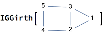
3
If the graph has no cycles, ∞ is returned.
IGGirth@IGShorthand["1-2"]∞
?IGDiameter
The diameter of a graph is the length of the longest shortest path between any two vertices.
The available options are:
Method can take the values
"Unweighted", "Dijkstra" or
Automatic. "Dijkstra" takes edge weights into
account. Automatic chooses based on whether the graph is
weighted.
"ByComponents" controls how unconnected graphs are
handled. If False, Infinity is returned. If
True, the longest shortest path is returned. In the
undirected case, this is the largest diameter of any connected
component.
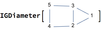
2
For the null graph, Indeterminate is returned.
IGDiameter[IGEmptyGraph[]]Indeterminate
?IGFindDiameter
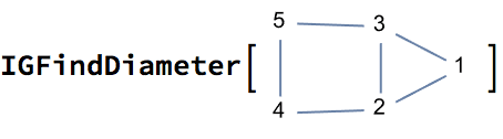
{1, 2, 4}
![]()
HighlightGraph[g, PathGraph@IGFindDiameter[g],
 GraphHighlightStyle -> "DehighlightFade", PlotTheme -> "RoyalColor"
 ]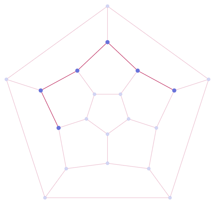
?IGEccentricity
The eccentricity of a vertex is the longest shortest path to any
other vertex. IGEccentricity computes the
unweighted eccentricity of each vertex within the connected
component where it is contained.
IGEccentricity@CycleGraph[8]{4, 4, 4, 4, 4, 4, 4, 4}
Connected components are considered separately.
IGEccentricity[IGDisjointUnion[{CycleGraph[3], CycleGraph[8]}]]{1, 1, 1, 4, 4, 4, 4, 4, 4, 4, 4}
?IGRadius
The radius of a graph is the smallest eccentricity of any of its vertices, i.e. the eccentricity of the graph center.
?IGVoronoiCells
IGVoronoiCells[graph, centers] partitions a graph’s
vertices into groups based on which given centre vertex they are the
closest to. Edge weights are considered for the distance
calculations.
Available options:
"Tiebreaker" sets the function used to decide which
cell a vertex should belong to if its distance to several different
centres is equal. The default is to use the first qualifying cell.
Possible useful settings are First, Last,
RandomChoice.g = PathGraph[Range[5], VertexLabels -> "Name", VertexSize -> Medium]![]()
IGVoronoiCells[g, {2, 4}]<|2 -> {1, 2, 3}, 4 -> {4, 5}|>
HighlightGraph[g, Values[%]]![]()
In the event of a tie, a vertex is added to the first qualifying cell. The tiebreaker function can be changed as below.
IGVoronoiCells[g, {2, 4}, "Tiebreaker" -> Last]<|2 -> {1, 2}, 4 -> {3, 4, 5}|>
Table[IGVoronoiCells[g, {2, 4}, "Tiebreaker" -> RandomChoice], {5}]{<|2 -> {1, 2, 3}, 4 -> {4, 5}|>, <|2 -> {1, 2}, 4 -> {3, 4, 5}|>, <|2 -> {1, 2, 3}, 4 -> {4, 5}|>, <|2 -> {1, 2, 3}, 4 -> {4, 5}|>, <|2 -> {1, 2}, 4 -> {3, 4, 5}|>}
Find Voronoi cells on a grid.
g = GridGraph[{10, 10}, VertexSize -> Medium,
   GraphStyle -> "BasicBlack"];
centers = RandomSample[VertexList[g], 3];
HighlightGraph[g,
 Append[
  Subgraph[g, #] & /@ Values@IGVoronoiCells[g, centers],
  Style[centers, Black]
  ],
 GraphHighlightStyle -> "DehighlightHide"
 ]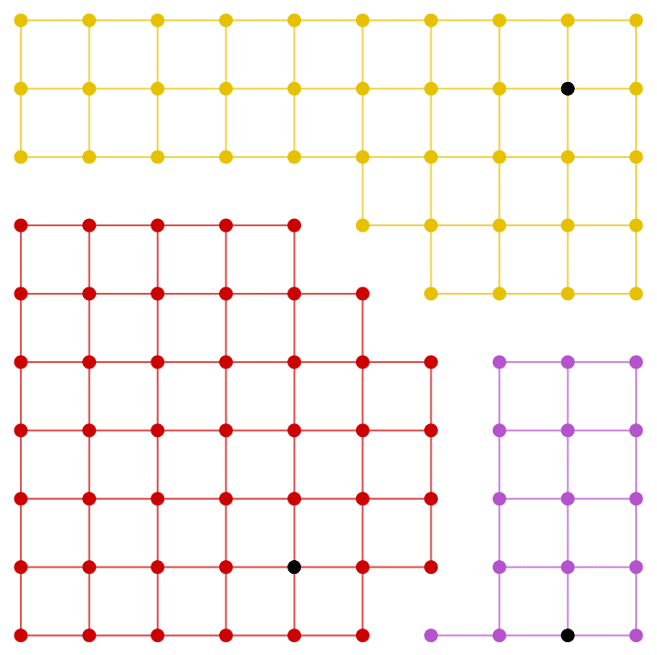
Edge weights are interpreted as distances.
g = IGMeshGraph@DelaunayMesh@RandomPoint[Disk[], 200];
centers = RandomSample[VertexList[g], 3];
HighlightGraph[g,
 Append[
  Subgraph[g, #] & /@ Values@IGVoronoiCells[g, centers],
  Style[centers, Black]
  ],
 GraphHighlightStyle -> "DehighlightGray"
 ]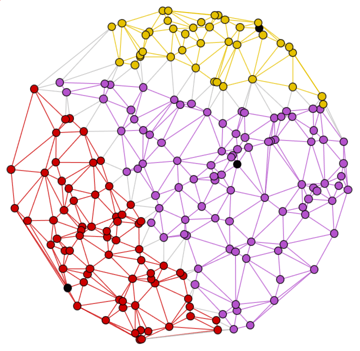
?IGShortestPathTree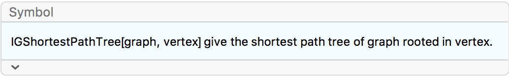
Experimental: This is experimental functionality that may change in the future.
g = IGTriangularLattice[4];HighlightGraph[g, IGShortestPathTree[g, 1],
GraphHighlightStyle -> "Thick"]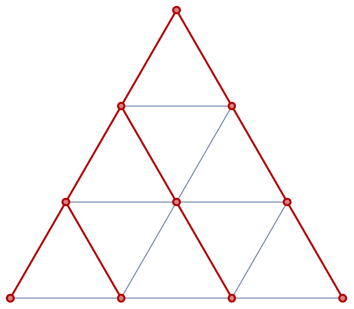
?IGGlobalEfficiency
IGGlobalEfficiency[graph] computes the global efficiency
of a graph. The global efficiency is defined as the average inverse
shortest path length between all pairs of vertices,
\[E_{\text{global}}=\frac{1}{V(V-1)}\sum _{u,v} \frac{1}{d_{uv}},\]
where \(d_{uv}\) is the graph distance from vertex \(u\) to vertex \(v\) and \(V\) is the number of vertices. When \(v\) is not reachable from \(u\), \(1\left/d_{uv}\right.\) is taken to be 0.
Available options:
DirectedEdges -> False ignores edge directions when
computing shortest path lengths.Compute the global efficiency of a network …
g = ExampleData[{"NetworkGraph", "ProteinInteraction"}];
IGGlobalEfficiency[g]
0.0997348
… and that of its spanning tree.
IGGlobalEfficiency@IGSpanningTree[g]0.00106384
?IGLocalEfficiency
IGLocalEfficiency[graph] computes the local efficiency
around each vertex of a graph. The local efficiency around a vertex
\(u\) is defined as the average
pairwise inverse shortest path length between the neighbours of \(u\) after excluding \(u\) itself from the graph,
\[E_{\text{local}}(u)=\frac{1}{k_u\left(k_u-1\right)}\sum _{v,w\in N(u)} \frac{1}{d_{vw}},\]
where \(k_u\) is the degree of vertex \(u\), \(N(u)\) denotes its neighbourhood and \(d_{vw}\) is the graph distance from vertex \(v\) to vertex \(w\). If \(u\) has less than two neighbours, \(E_{\text{local}}(u)\) is taken to be 0.
Available options:
DirectedEdges -> False ignores edge directions when
computing shortest path lengths.Size the vertices of a graph according to the corresponding local efficiency
g = ExampleData[{"NetworkGraph", "ZacharyKarateClub"}];
IGVertexMap[1.5 # &, VertexSize -> IGLocalEfficiency, g]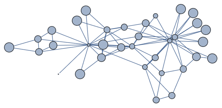
Plot the local efficiency versus the local clustering coefficient.
ListPlot[
 Transpose[{IGLocalClusteringCoefficient[g], IGLocalEfficiency[g]}],
 PlotTheme -> "Detailed"
 ]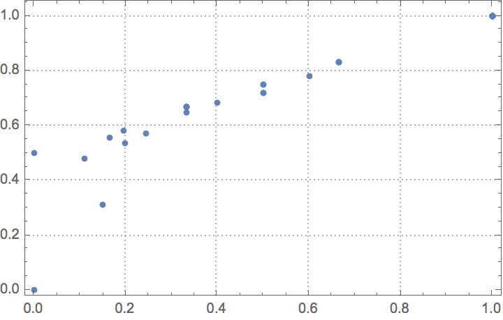
Compute the local efficiency of a subset of vertices only.
g = RandomGraph[{10, 20}, DirectedEdges -> True];
IGLocalEfficiency[g, {1, 2, 3}]{0.506944, 0.408333, 0.5}
By default, both in- and out-neighbours are considered when determining the neighbourhoods of vertices. We can also consider only in-neighbours or only out-neighbours.
{IGLocalEfficiency[g, All, "All"],
 IGLocalEfficiency[g, All, "In"],
IGLocalEfficiency[g, All, "Out"]}{{0.506944, 0.408333, 0.5, 0.388889, 0.275, 0.305556, 0.375, 0.336111, 0.493333, 0.35}, {1., 0.625, 0.5, 0.5, 0.25, 0.25, 0.375, 0.1, 0.416667, 0.}, {0.125, 0., 0., 0.25, 0.388889, 0.25, 0., 0.5, 0.520833, 0.35}}
Ignore edge directions when computing shortest paths.
IGLocalEfficiency[g, DirectedEdges -> False]{0.722222, 0.833333, 1., 0.75, 0.561667, 0.5, 0.583333, 0.583333, \ 0.7, 0.5}
?IGAverageLocalEfficiency
IGAverageLocalEfficiency[graph] computes the average
local efficiency of a network. See IGLocalEfficiency for a
definition of this graph measure.
Plot the decrease in average local efficiency during sequential edge removals.
g = RandomGraph[{30, 60}, DirectedEdges -> True];ListPlot[
Table[
{k, IGAverageLocalEfficiency@
Graph[VertexList[g], Take[EdgeList[g], k]]},
{k, EdgeCount[g]}
],
AxesLabel -> {"edge count", "local efficiency"}
]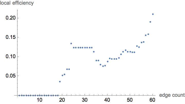
IGAverageLocalEfficiency simply gives the average of the
values returned by IGLocalEfficiency.
{IGAverageLocalEfficiency[g], Mean@IGLocalEfficiency[g]}{0.210095, 0.210095}
Use only the out-neighbourhood while computing the local efficiency.
IGAverageLocalEfficiency[g, "Out"]0.142476
The vertices of a bipartite graph can be divided into two groups (partitions) such that connections run only between the two partitions, but never within a single partition.
?IGBipartite*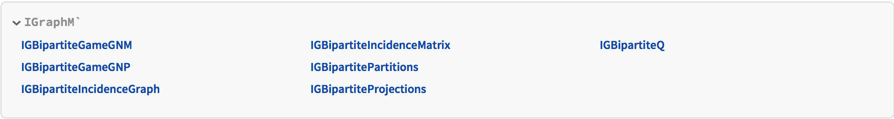
?IGBipartiteQ
Generate a graph and verify that it is bipartite.
g = IGBipartiteGameGNM[5, 5, 10, VertexLabels -> "Name"]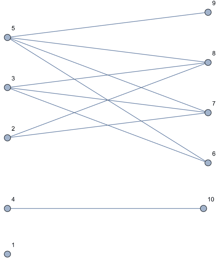
IGBipartiteQ[g]True
Verify that no edges run between two disjoint vertex subsets of the graph.
IGBipartiteQ[g, {{1, 2, 3}, {6, 7, 8}}]True
?IGBipartitePartitions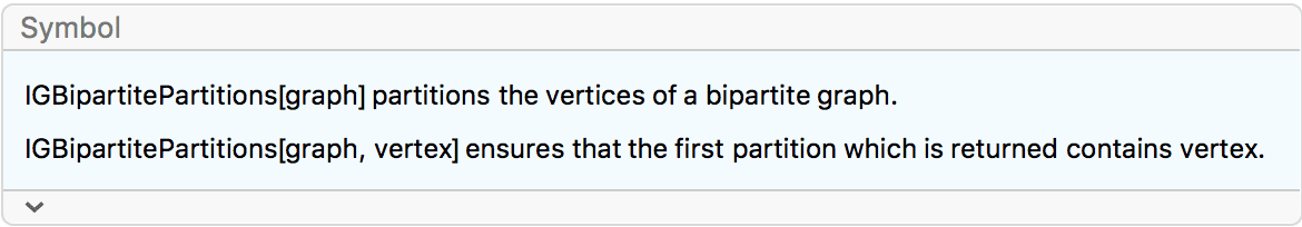
Find a bipartite partitioning of a graph.
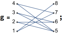
IGBipartitePartitions[g]{{1, 2, 3, 4}, {5, 6, 7, 8}}
Ensure that the partitions are returned in such an order that the first one contains vertex 5.
IGBipartitePartitions[g, 5]{{5, 6, 7, 8}, {1, 2, 3, 4}}
$Failed is returned for non-bipartite graphs.
IGBipartitePartitions[CompleteGraph[4]]![]()
$Failed
We can use IGPartitionsToMembership or
IGKVertexColoring[…, 2] to obtain a partition index for
each vertex.
IGPartitionsToMembership[g]@IGBipartitePartitions[g]{1, 1, 1, 1, 2, 2, 2, 2}
IGKVertexColoring[g, 2]{{1, 1, 1, 1, 2, 2, 2, 2}}
?IGBipartiteProjections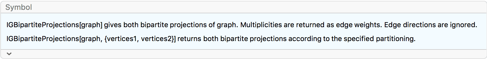
The following bipartite graph described the relationship between diseases and genes.
g = ExampleData[{"NetworkGraph", "BipartiteDiseasomeNetwork"}]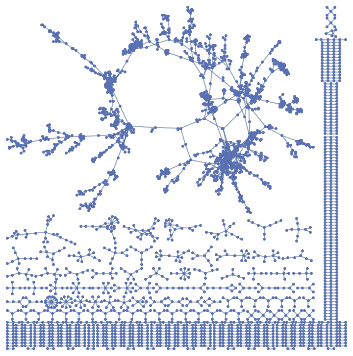
parts = Values@GroupBy[
    Thread[IGVertexProp["Type"][g] -> VertexList[g]],
    First -> Last
    ];
Construct a disease-disease and gene-gene network from it.
IGBipartiteProjections[g, parts]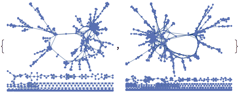
?IGBipartiteIncidenceGraph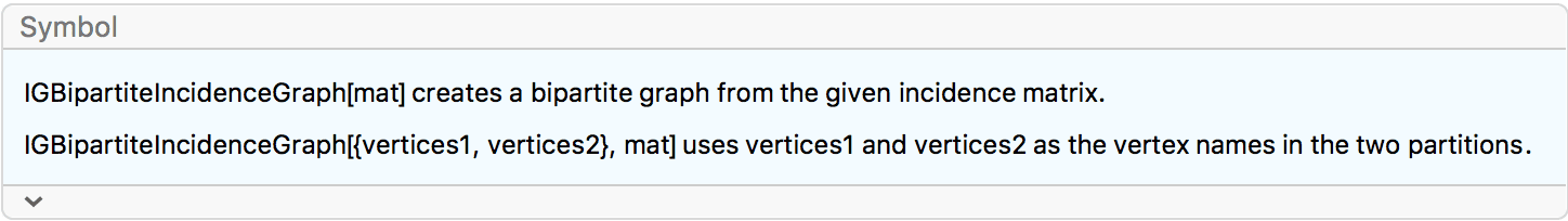
?IGBipartiteIncidenceMatrix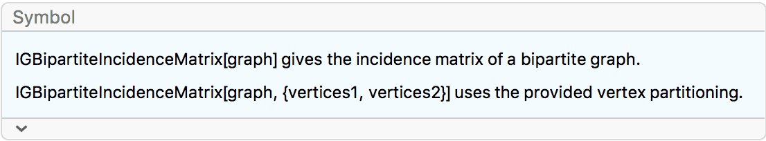
Compute an incidence matrix. The default partitioning used by
IGBipartiteIncidenceMatrix is the one returned by
IGBipartitePartitions.
g = IGBipartiteGameGNM[5, 5, 10, VertexLabels -> "Name"]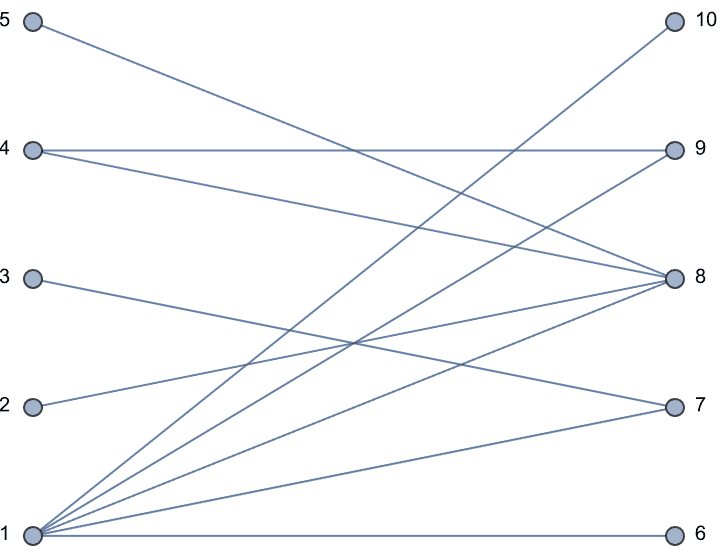
bm = IGBipartiteIncidenceMatrix[g];
MatrixForm[bm, TableHeadings -> IGBipartitePartitions[g]]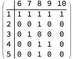
Reconstruct a graph from an incidence matrix.
IGBipartiteIncidenceGraph[bm, VertexLabels -> "Name",
 GraphLayout -> "BipartiteEmbedding"]
Compute an incidence matrix using a given partitioning / vertex ordering. It is allowed to pass only a subset of vertices.
IGBipartiteIncidenceMatrix[g, {{1, 2, 3}, {6, 7, 8}}]![]()
Reconstruct the bipartite graph while specifying vertex names.
IGBipartiteIncidenceGraph[{{a, b, c}, {d, e, f}}, %,
 VertexLabels -> "Name"]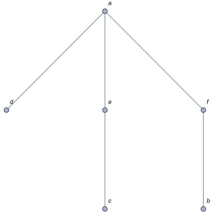
The functions in this section characterize the similarity of vertex pairs within a graph.
?IGBibliographicCoupling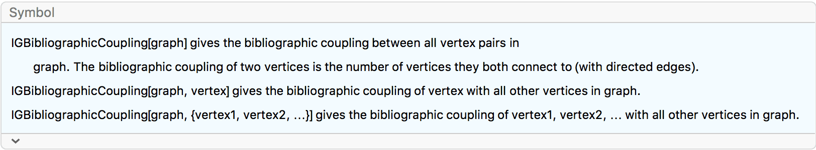
The bibliographic coupling of two vertices in a directed graph is the
number of other vertices they both connect to. The bibliographic
coupling matrix can also be obtained using
am . am\[Transpose] - DiagonalMatrix@VertexInDegree[g],
where am is the adjacency matrix of the graph
g.
?IGStaticPowerLawGame
Create a random graph and compute its bibliographic coupling matrix.
g = IGStaticPowerLawGame[10, 25, 2, 4,
  GraphLayout -> "CircularEmbedding", GraphStyle -> "BasicBlack"]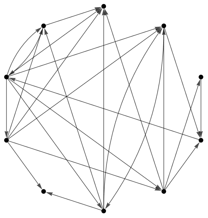
cc = IGBibliographicCoupling[g];
MatrixForm[cc, TableHeadings -> {VertexList[g], VertexList[g]}]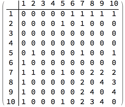
Construct the weighted graph corresponding to the bibliographic coupling of vertices and visualize it.
ccg = IGWeightedAdjacencyGraph[cc,
   VertexCoordinates -> GraphEmbedding[g],
   GraphStyle -> "ThickEdge"] //
  IGEdgeMap[Thickness[0.02 #] &, EdgeStyle -> IGEdgeProp[EdgeWeight]]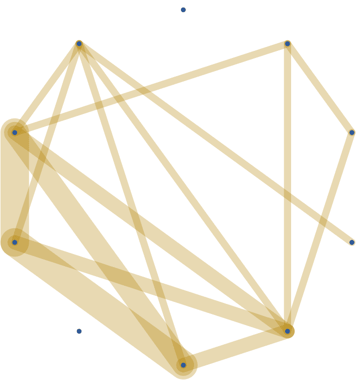
Overlay the bibliographic coupling graph with the original directed graph.
Show[ccg, g]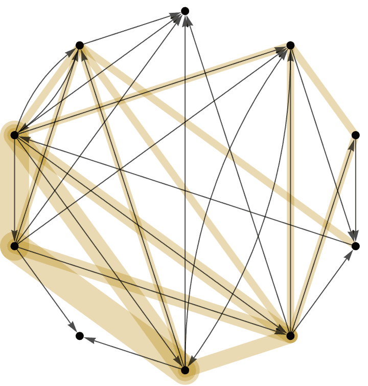
?IGCocitationCoupling
The co-citation coupling of two vertices in a directed graph is the
number of other vertices that connect to both of them. The co-citation
coupling matrix can also be obtained using
am\[Transpose] . am - DiagonalMatrix@VertexOutDegree[g],
where am is the adjacency matrix of the graph
g.
?IGDiceSimilarity
The Dice similarity coefficient of two vertices is twice the number of common neighbours divided by the sum of the degrees of the vertices. For directed graphs, out-neighbours are considered. Edge multiplicities are not taken into account.
The available options are:
SelfLoops -> True will include self-loops in the
calculation of the similarity score.?IGJaccardSimilarity
The Jaccard similarity coefficient of two vertices is the number of common neighbours divided by the number of vertices that are neighbours of at least one of the two vertices being considered. For directed graphs, out-neighbours are considered. Edge multiplicities are not taken into account.
The available options are:
SelfLoops -> True will include self-loops in the
calculation of the similarity score.Construct and visualize a weighted graph of Jaccard similarities between vertices of an animal social network:
g = ExampleData[{"NetworkGraph", "DolphinSocialNetwork"}]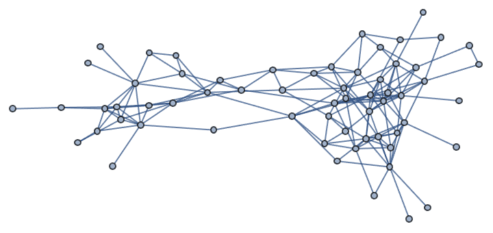
IGWeightedAdjacencyGraph[IGZeroDiagonal@IGJaccardSimilarity[g],
  VertexCoordinates -> GraphEmbedding[g]] //
 IGEdgeMap[GrayLevel[0, #] &, EdgeStyle -> IGEdgeProp[EdgeWeight]]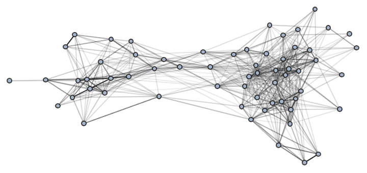
Compare it to the inverse log-weighted similarity:
IGWeightedAdjacencyGraph[Rescale@IGInverseLogWeightedSimilarity[g],
  VertexCoordinates -> GraphEmbedding[g]] //
 IGEdgeMap[GrayLevel[0, #] &, EdgeStyle -> IGEdgeProp[EdgeWeight]]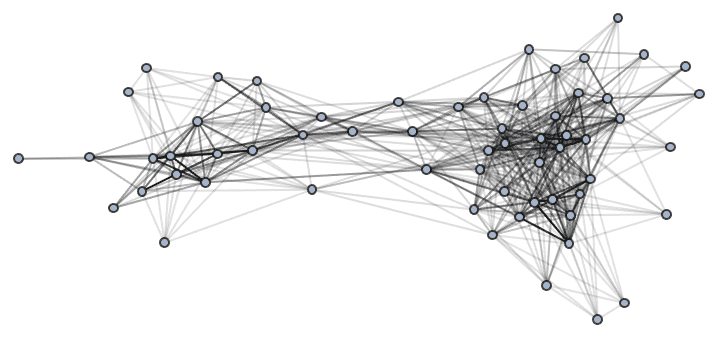
?IGInverseLogWeightedSimilarity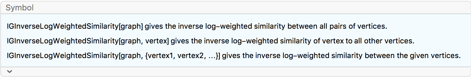
The inverse log-weighted similarity of two vertices is the number of their common neighbours, weighted by the inverse natural logarithm of the neighbours’ degrees. It is also known as the Adamic–Adar index. It is based on the assumption that two vertices should be considered more similar if they share a low-degree common neighbour, since high-degree common neighbours are more likely to appear even by pure chance.
Formally, the similarity of vertices \(u\) and \(v\) is
\[A(u,v)=\sum _{w\in \mathcal{N}(u)\cap \mathcal{N}(v)} \frac{1}{\ln d_w},\]
where \(\mathcal{N}(u)\) denotes the neighbourhood of vertex \(u\) and \(d_w\) denotes the degree of vertex \(w\).
Isolated vertices will have zero similarity to any other vertex. Self-similarities are not calculated.
In directed graphs, the out-neighbours of each vertex are considered, weighted by the inverse logarithm of their in-degrees.
?IGConnectedQ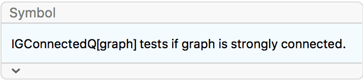
?IGWeaklyConnectedQ
IGConnectedQ checks if the graph is (strongly)
connected. It is equivalent to ConnectedGraphQ.
IGWeaklyConnectedQ check if a directed graph is weakly
connected. It is equivalent to WeaklyConnectedGraphQ. Both
of these functions use the implementation from the core igraph library,
and will always be consistent with it for edge cases such as the null
graph.
This graph is connected.
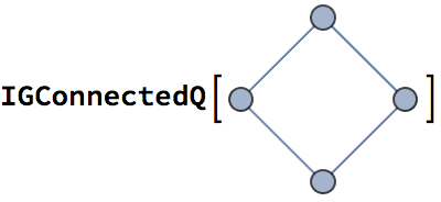
True
This directed graph is only weakly connected.
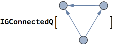
False
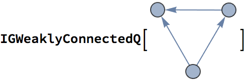
True
The null graph is considered disconnected by convention.
IGConnectedQ@IGEmptyGraph[0]False
?IGConnectedComponentSizes
?IGWeaklyConnectedComponentSizes
IGWeaklyConnectedComponentsSizes and
IGConnectedComponentSizes return the sizes of the graph’s
weakly or strongly connected components in decreasing order.
In large graphs, these functions will be faster than the equivalent
Length /@ ConnectedComponents[g].
The emergence of a giant component as the number of edges in a random graph increases.
Table[
  {m, First@IGConnectedComponentSizes@RandomGraph[{1000, m}]},
  {m, 5, 2000, 5}
  ] // ListPlot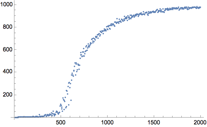
The number of weakly and strongly connected components versus the number of edges in a random directed graph.
Table[
   With[{g = RandomGraph[{1000, m}, DirectedEdges -> True]},
    {{m, Length@IGWeaklyConnectedComponentSizes[g]}, {m,
      Length@IGConnectedComponentSizes[g]}}
    ],
   {m, 5, 3000, 5}
   ] // Transpose // ListPlot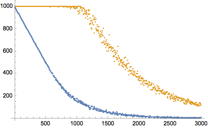
?IGFindMinimumCuts
IGFindMinimalCuts[g, s, t] finds all **smallest-weight
(i.e. minimum) edge cuts that disconnect vertex t from
vertex s.
g = ExampleData[{"NetworkGraph", "MetabolicNetworkAeropyrumPernix"}];
IGFindMinimumCuts[g, 30, 160]{{30 \[DirectedEdge] 1000177, 30 \[DirectedEdge] 1000178}, {30 \[DirectedEdge] 1000178, 1000177 \[DirectedEdge] 10}, {1000080 \[DirectedEdge] 160, 1000092 \[DirectedEdge] 160}}
Visualize all minimum cuts between two vertices in a random cubic graph.
g = IGKRegularGame[20, 3];
HighlightGraph[g, Join[#, {1, 20}], GraphHighlightStyle -> "Dotted",
   VertexSize -> Large] & /@ IGFindMinimumCuts[g, 1, 20]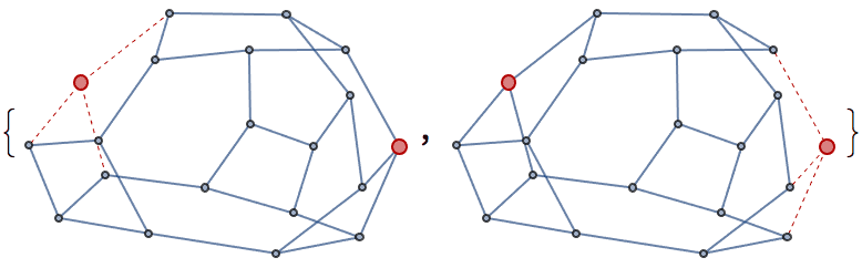
Warning: IGFindMinimumCuts takes edge
weights into account, but it is only safe to use with integer weights.
If the weights are not integers, then numerical roundoff errors may
prevent the function from detecting that two cuts have the same total
weight.
Create an integer-weighted graph with more than one minimum cut
between vertices 1 and 10:
g = IGTryUntil[Length@IGFindMinimumCuts[#, 1, 10] > 2 &][
  RandomGraph[{10, 30}, DirectedEdges -> True,
   EdgeWeight -> RandomInteger[{1, 10}, 30]]]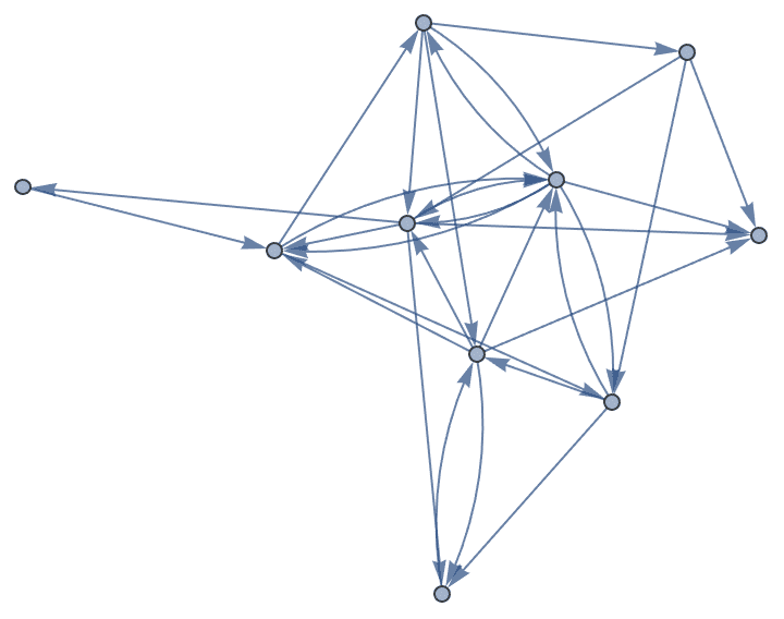
IGFindMinimumCuts[g, 1, 10]{{1 \[DirectedEdge] 3, 1 \[DirectedEdge] 6, 1 \[DirectedEdge] 7, 1 \[DirectedEdge] 8}, {1 \[DirectedEdge] 3, 2 \[DirectedEdge] 3, 2 \[DirectedEdge] 10, 4 \[DirectedEdge] 10}, {2 \[DirectedEdge] 10, 3 \[DirectedEdge] 10, 4 \[DirectedEdge] 10}}
Multiplying the weights by 0.1 causes
IGFindMinimumCuts to return fewer results because some of
the weights are no longer exactly representable in binary:
IGFindMinimumCuts[IGEdgeMap[0.1 # &, EdgeWeight, g], 1, 10]{{1 \[DirectedEdge] 3, 1 \[DirectedEdge] 6, 1 \[DirectedEdge] 7, 1 \[DirectedEdge] 8}}
If only a single minimum cut is needed, use
IGMinimumCut:
IGMinimumCut[g, 1, 10]{2 \[DirectedEdge] 10, 3 \[DirectedEdge] 10, 4 \[DirectedEdge] 10}
The size (total weight) of the cut can be obtained with
IGMinimumCutValue:
IGMinimumCutValue[g, 1, 10]14.
?IGFindMinimalCuts
IGFindMinimalCuts[g, s, t] finds all unweighted
minimal edge cuts that disconnect vertex t from vertex
s.
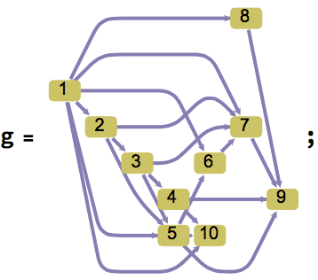
IGFindMinimalCuts[g, 1, 10]{{1 \[DirectedEdge] 2, 1 \[DirectedEdge] 5, 1 \[DirectedEdge] 10}, {1 \[DirectedEdge] 2, 1 \[DirectedEdge] 10, 5 \[DirectedEdge] 10}, {1 \[DirectedEdge] 5, 1 \[DirectedEdge] 10, 2 \[DirectedEdge] 3, 2 \[DirectedEdge] 5}, {1 \[DirectedEdge] 10, 2 \[DirectedEdge] 3, 5 \[DirectedEdge] 10}, {1 \[DirectedEdge] 5, 1 \[DirectedEdge] 10, 2 \[DirectedEdge] 5, 3 \[DirectedEdge] 4, 3 \[DirectedEdge] 5}, {1 \[DirectedEdge] 10, 3 \[DirectedEdge] 4, 5 \[DirectedEdge] 10}, {1 \[DirectedEdge] 5, 1 \[DirectedEdge] 10, 2 \[DirectedEdge] 5, 3 \[DirectedEdge] 5, 4 \[DirectedEdge] 10}, {1 \[DirectedEdge] 10, 4 \[DirectedEdge] 10, 5 \[DirectedEdge] 10}}
The set of all minimum cuts is a subset of the minimal ones.
IGFindMinimumCuts[g, 1, 10]{{1 \[DirectedEdge] 2, 1 \[DirectedEdge] 5, 1 \[DirectedEdge] 10}, {1 \[DirectedEdge] 2, 1 \[DirectedEdge] 10, 5 \[DirectedEdge] 10}, {1 \[DirectedEdge] 10, 2 \[DirectedEdge] 3, 5 \[DirectedEdge] 10}, {1 \[DirectedEdge] 10, 3 \[DirectedEdge] 4, 5 \[DirectedEdge] 10}, {1 \[DirectedEdge] 10, 4 \[DirectedEdge] 10, 5 \[DirectedEdge] 10}}
SubsetQ[%%, %]True
Visualize all minimal cuts between two vertices, from smallest to largest, in an undirected graph.
g = IGGiantComponent@RandomGraph[{8, 12}];
HighlightGraph[g, Join[#, {1, 8}], GraphHighlightStyle -> "Dashed",
   VertexSize -> Medium] & /@
 SortBy[Length]@IGFindMinimalCuts[g, 1, 8]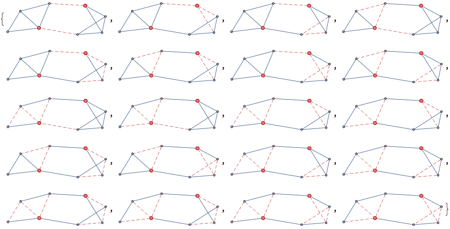
A vertex separator is a set of vertices whose removal disconnects the graph.
?IGMinimalSeparators
?IGMinimumSeparators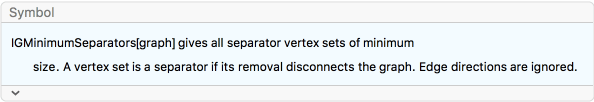
?IGVertexSeparatorQ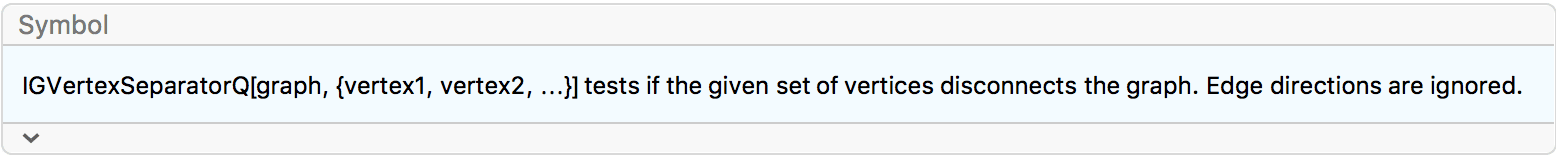
?IGMinimalVertexSeparatorQ
g = ExampleData[{"NetworkGraph", "Friendship"}]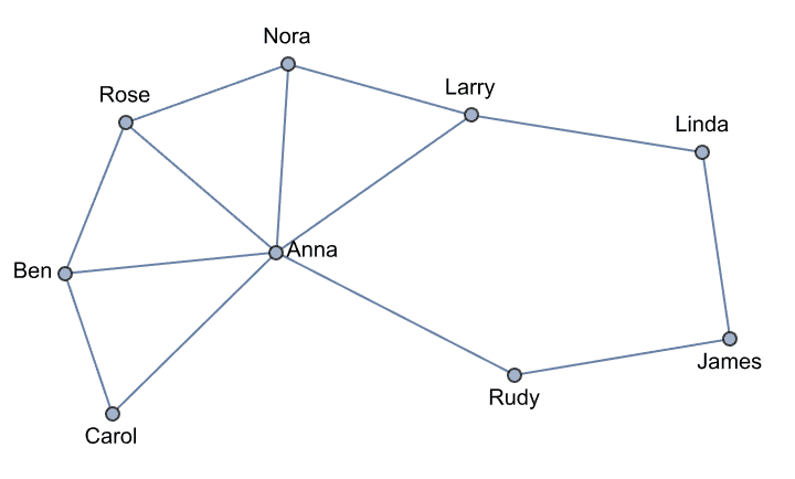
separators = IGMinimumSeparators[g]{{"Anna", "Rose"}, {"Larry", "Rudy"}, {"Larry", "James"}, {"Rudy", "Linda"}, {"Anna", "Nora"}, {"Anna", "Ben"}, {"Anna", "Larry"}, {"Anna", "Linda"}, {"Anna", "James"}}
Removing any of these vertex sets will disconnect the graph:
VertexDelete[g, #] & /@ separators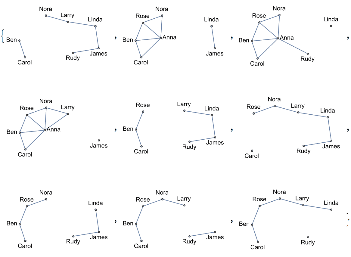
IGVertexSeparatorQ[g, #] & /@ separators{True, True, True, True, True, True, True, True, True}
IGMinimalVertexSeparatorQ[g, #] & /@ separators{True, True, True, True, True, True, True, True, True}
Removing Anna, Nora and Larry also disconnects the graph, thus this vertex set is a separator:
IGVertexSeparatorQ[g, {"Anna", "Nora", "Larry"}]True
But it is not minimal:
IGMinimalVertexSeparatorQ[g, {"Anna", "Nora", "Larry"}]False
IGMinimumSeparators returns only those vertex separators
which are of the smallest possible size in the graph.
IGMinimalSeparators returns all separators which cannot be
made smaller by removing a vertex from them. The former is a subset of
the latter.
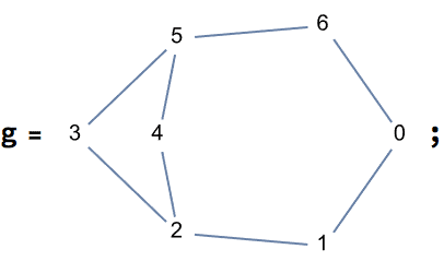
IGMinimalSeparators[g]{{1, 6}, {0, 2}, {1, 3, 4}, {2, 5}, {3, 4, 6}, {0, 5}, {2, 6}, {1, 5}, {0, 3, 4}}
IGMinimumSeparators[g]{{2, 5}, {1, 5}, {1, 6}, {0, 5}, {2, 6}, {0, 2}}
SubsetQ[%%, %]True
?IGEdgeConnectivity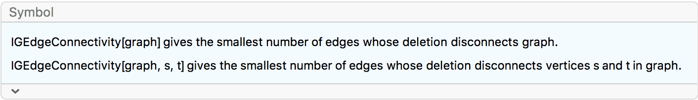
IGEdgeConnectivity ignores edge weights. To take edge
weights into account, use IGMinimumCutValue instead.
Compute the edge connectivity of the dodecahedral graph.
IGEdgeConnectivity[GraphData["DodecahedralGraph"]]3
The edge connectivity of the singleton graph is returned as 0.
IGEdgeConnectivity[IGEmptyGraph[1]]0
?IGVertexConnectivity
According to Steinitz’s theorem, the skeleton of every convex polyhedron is a 3-vertex-connected planar graph.
g = GraphData["DodecahedralGraph"]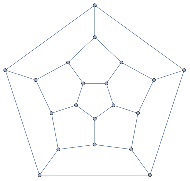
IGVertexConnectivity[g]3
To find the specific vertex sets that disconnect the graph, use
IGMinimumSeparators or
IGMinimalSeparators.
IGMinimumSeparators[g]{{14, 15, 16}, {5, 6, 13}, {7, 14, 19}, {8, 15, 20}, {2, 11, 19}, {2, 12, 20}, {3, 11, 16}, {4, 12, 16}, {10, 14, 17}, {9, 15, 18}, {5, 7, 12}, {6, 8, 11}, {2, 17, 18}, {9, 13, 19}, {10, 13, 20}, {3, 5, 17}, {4, 6, 18}, {1, 3, 9}, {1, 4, 10}, {1, 7, 8}}
The vertex connectivity of the singleton graph is returned as 0.
IGVertexConnectivity[IGEmptyGraph[1]]0
?IGBiconnectedQ
IGBiconnectedQ checks if a graph is biconnected. Edge
directions are ignored.
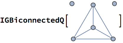
False
Since IGBiconnectedComponents does not return any
isolated vertices, Length@IGBiconnectedComponents[g] == 1
cannot be used to check if a graph is biconnected. Use
IGBiconnectedQ instead.
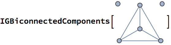
{{4, 3, 2, 1}}
The singleton graph is not considered to be biconnected, but the two-vertex complete graph is.
Table[IGBiconnectedQ@CompleteGraph[k], {k, 1, 2}]{False, True}
?IGBiconnectedComponents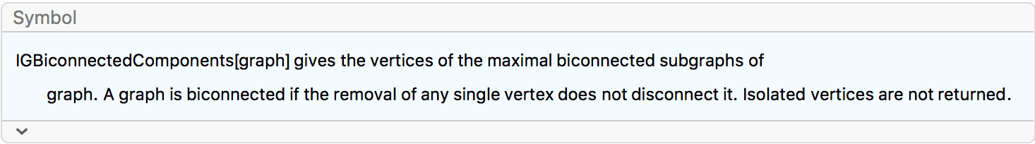
?IGBiconnectedEdgeComponents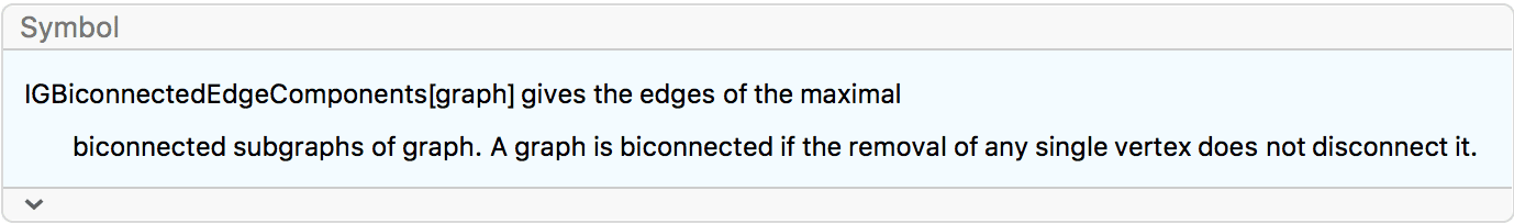
IGBiconnectedCompoments returns the vertices of the
maximal biconnected components of the graph.
IGBiconnectedEdgeComponents returns the edges of the
components. Edge directions are ignored and isolated vertices are
excluded.
IGBiconnectedComponents is equivalent to
KVertexConnectedComponents[…, 2], except that isolated
vertices are not returned as individual components.
The articulation vertices will be part of more than a single component, thus the biconnected components are not disjoint subsets of the vertex set.
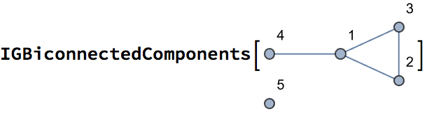
{{3, 2, 1}, {4, 1}}
However, each edge is part of precisely one biconnected components.
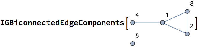
{{1 <-> 3, 2 <-> 3,
 1 <-> 2}, {1 <-> 4}}
Thus, visualizing biconnected components is best done by colouring the edges, not the vertices.
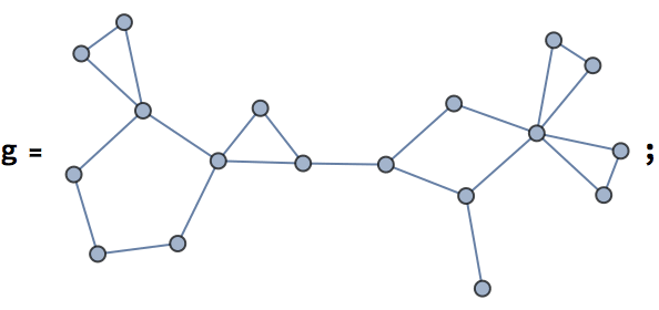
HighlightGraph[g, IGBiconnectedEdgeComponents[g],
 GraphStyle -> "ThickEdge"]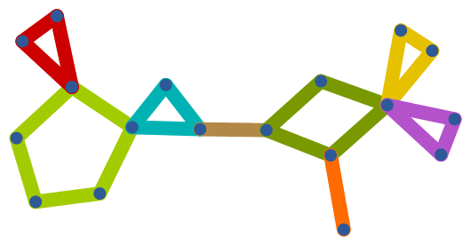
?IGArticulationPoints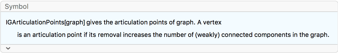
IGArticulationPoints finds vertices whose removal
increases the number of (weakly) connected components in the graph. Edge
directions are ignored.
g = Graph[{1 -> 2, 2 -> 3, 3 -> 1, 3 -> 4, 4 -> 5, 5 -> 6, 6 -> 4},
  DirectedEdges -> False, VertexLabels -> Automatic]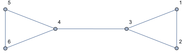
IGArticulationPoints[g]{4, 3}
VertexDelete[g, #] & /@ %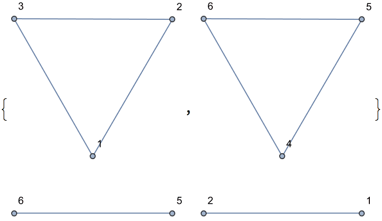
Articulation points are also size-1 separators.
IGMinimumSeparators[g]{{4}, {3}}
Highlight the articulation points of a cactus graph.
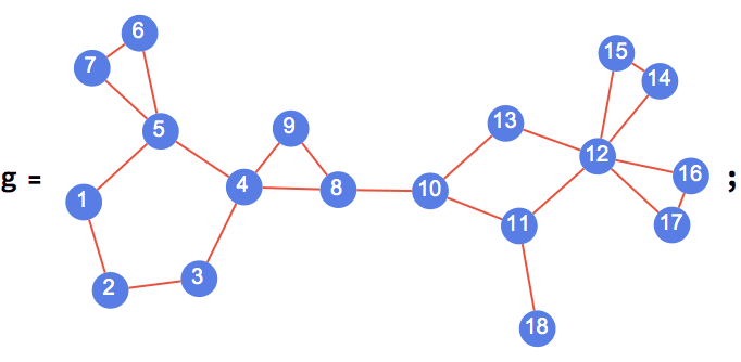
HighlightGraph[g, IGArticulationPoints[g]]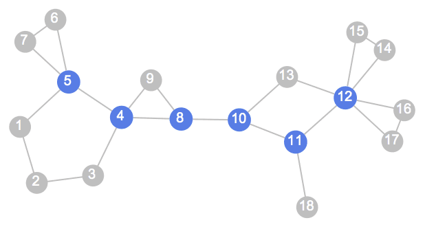
Compute the block-cut tree of a connected graph. The blocks are the biconnected components. Together with the articulation vertices they form a bipartite graph, specifically a tree.
RelationGraph[
 MemberQ,
 Join[IGBiconnectedComponents[g], IGArticulationPoints[g]],
 DirectedEdges -> False,
 GraphStyle -> "ClassicDiagram",
 VertexSize -> {3, 1}/7, VertexLabelStyle -> 8
 ]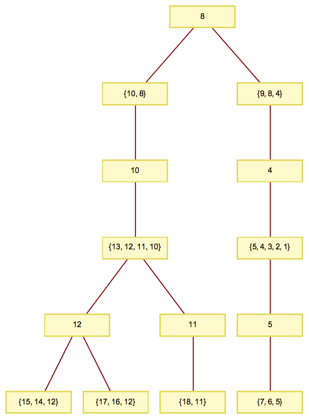
?IGBridges
A bridge is an edge whose removal disconnects the graph (or increases the number of connected components if the graph was already disconnected). Edge directions are ignored.
IGShorthand["1-2-3-1-4-5-6-4"]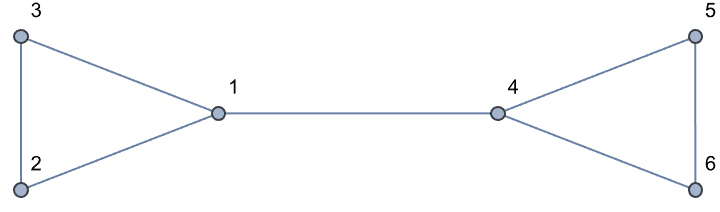
IGBridges[%]{1 <-> 4}
Highlight bridges in a network.
g = ExampleData[{"NetworkGraph", "FlorentineFamilies"}];
HighlightGraph[g, IGBridges[g]]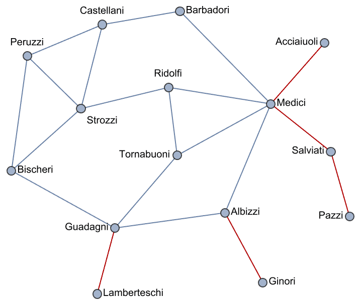
?IGSourceVertexList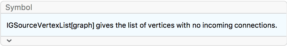
?IGSinkVertexList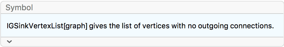
Find and highlight the source and sink vertices of a random acyclic graph.
g = DirectedGraph[RandomGraph[{10, 20}], "Acyclic",
  VertexLabels -> "Name", VertexSize -> Large, EdgeStyle -> Gray]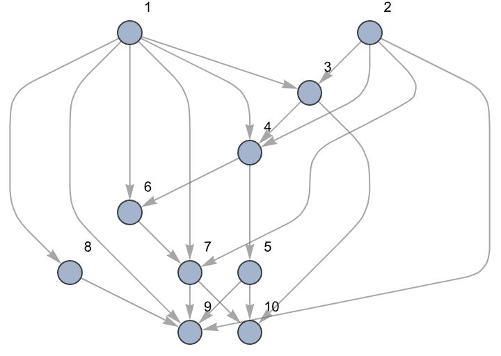
IGSourceVertexList[g]{1, 2}
IGSinkVertexList[g]{9, 10}
HighlightGraph[g, {IGSourceVertexList[g], IGSinkVertexList[g]}]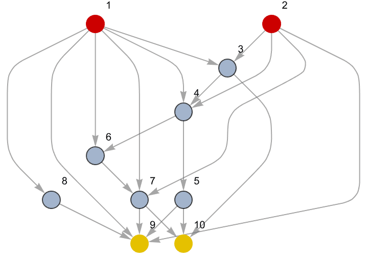
Undirected graphs have neither source nor sink vertices because undirected edges are counted as bidirectional.
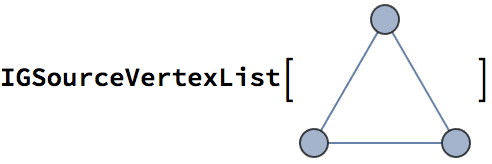
{}
The exception is isolated vertices, which are counted both as sources and sinks.
Through[{IGSourceVertexList, IGSinkVertexList}@Graph[{1, 2}, {}]]{{1, 2}, {1, 2}}
These are merely convenience functions that can be implemented straightforwardly as
Pick[VertexList[g], VertexOutDegree[g], 0]{9, 10}
?IGIsolatedVertexList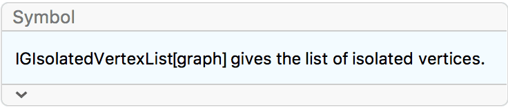
IGIsolatedVertexList returns the vertices which form
their own weakly connected components. This includes vertices with no
connections, as well as vertices with only self-loops.
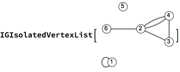
{1, 5}
?IGGiantComponent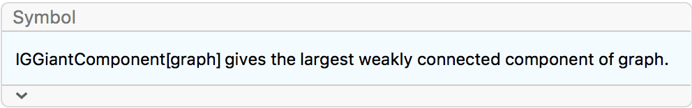
IGGiantComponent is a convenience function that returns
the largest weakly connected component of graph. If there are multiple
components of largest size, there is no guarantee about which one would
be returned. If this is a concern, use
WeaklyConnectedComponents or
WeaklyConnectedGraphComponents instead.
g = RandomGraph[{200, 200}];
HighlightGraph[
  g,
  IGGiantComponent[g]
  ] // IGLayoutFruchtermanReingold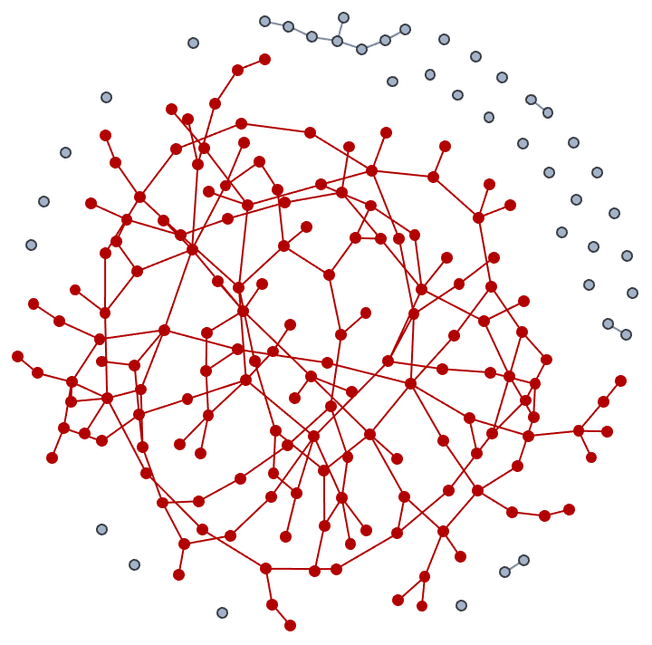
IGGiantComponent takes all standard graph options.
IGGiantComponent[g, GraphStyle -> "BasicGreen",
 GraphLayout -> "SpringEmbedding"]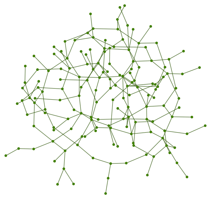
Size of the giant component of a random subgraph of a grid graph.
g = IGSquareLattice[{30, 30}, "Periodic" -> True];
Table[
  {k, VertexCount@
    IGGiantComponent@Subgraph[g, RandomSample[VertexList[g], k]]},
  {k, 1, VertexCount[g], 1}
  ] // ListPlot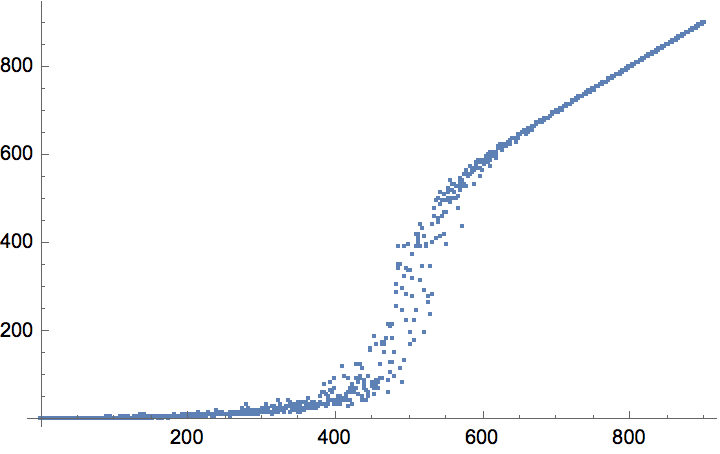
?IGPercolationCurve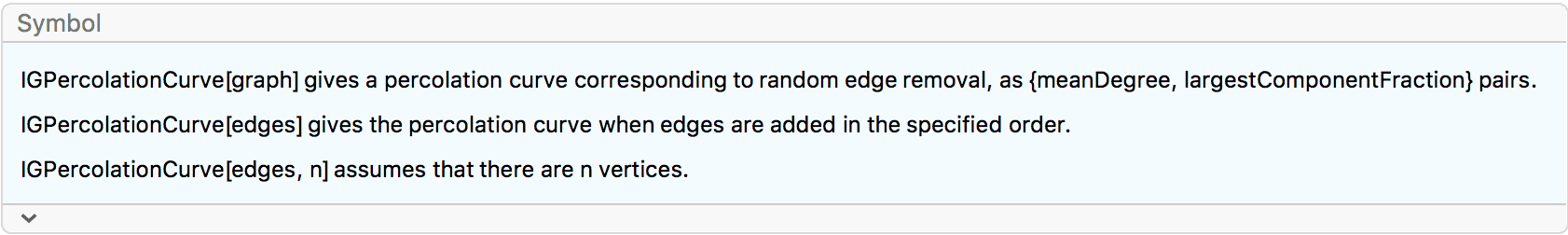
Experimental: This is experimental functionality that may change in the future.
IGPercolationCurve computes the percolation curve for a
sequence of edge additions (interpretable as edge removals in reverse
order). The ith element of the result is the mean degree
and the fraction of vertices within the largest component before adding
the ith edge.
IGPercolationCurve[graph] is equivalent to
IGPercolationCurve[RandomSample@EdgeList[graph], VertexCount[graph]].
Plot the averaged percolation curve of a grid graph over many random edge removals.
ListLinePlot@Mean@Table[IGPercolationCurve@GridGraph[{50, 50}], {100}]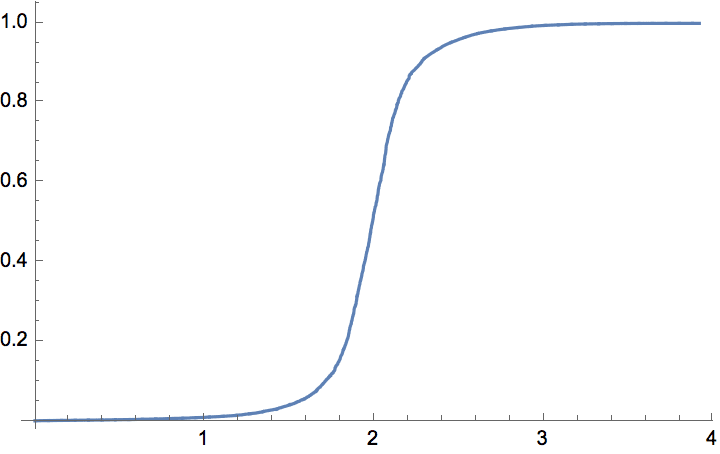
Percolation curve for a random geometric graph when edges are removed in order of decreasing or increasing betweenness.
g = IGGeometricGame[500, 0.1];
edgeOrder = EdgeList[g][[Ordering@IGEdgeBetweenness[g]]];ListLinePlot[IGPercolationCurve /@ {edgeOrder, Reverse[edgeOrder]},
PlotLegends -> {"decreasing betweenness", "increasing betweenness"},
FrameLabel -> {"mean degree", "largest component fraction"},
Frame -> True, PlotRange -> All]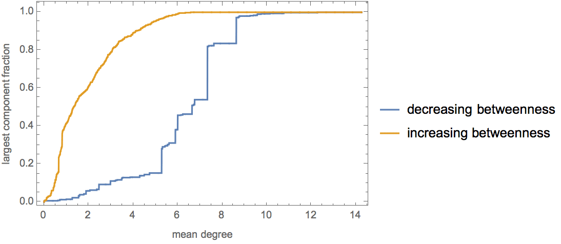
IGPercolationCurve also accepts a list of pairs in
addition to a list of edge expressions.
IGPercolationCurve@RandomInteger[{1, 10}, {20, 2}]{{0., 0.1}, {0., 0.2}, {0.2, 0.2}, {0.4, 0.2}, {0.6, 0.2}, {0.8, 0.3}, {1., 0.4}, {1.2, 0.4}, {1.4, 0.6}, {1.6, 0.7}, {1.8, 0.7}, {2., 0.9}, {2.2, 0.9}, {2.4, 1.}, {2.6, 1.}, {2.8, 1.}, {3., 1.}, {3.2, 1.}, {3.4, 1.}, {3.6, 1.}, {3.8, 1.}}
IGPercolationCurve works efficiently on large
networks.
g = ExampleData[{"NetworkGraph", "WorldWideWeb"}];
EdgeCount[g]
1497134
ListLinePlot[IGPercolationCurve[g], MaxPlotPoints -> 1000]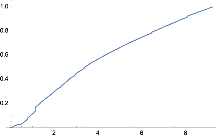
A tree is a connected graph that contains no undirected cycles.
?IGTreeQ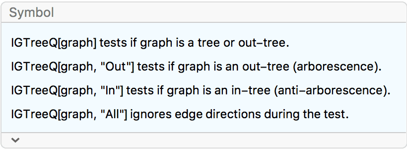
IGTreeQ checks if a graph is a tree. An undirected tree
is a connected graph with no cycles. A directed tree is similar, with
its edges oriented either away from a root vertex (out-tree or
arborescence) or towards a root vertex (in-tree or
anti-arborescence).
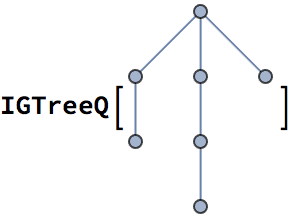
True
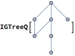
False
By convention, the null graph is not a tree.
IGTreeQ[IGEmptyGraph[0]]False
This is an out-tree.
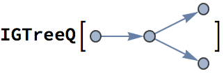
True
It is not also an in-tree.
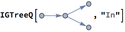
False
It becomes an in-tree if we reverse its edges.
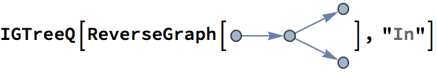
True
This graph is neither an out-tree nor an in-tree.
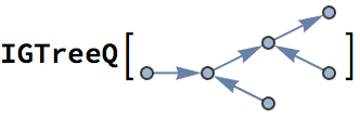
False
However, it becomes a tree if we ignore edge directions.
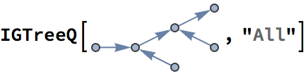
True
?IGForestQ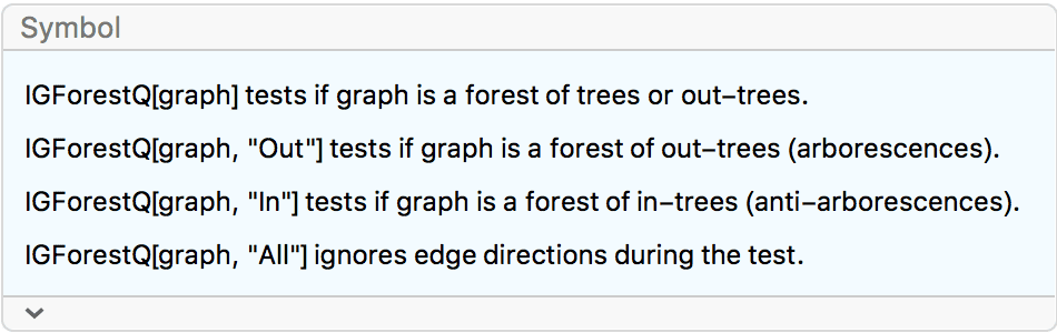
IGForestQ is a convenience function that tests if all
connected components of a graph are trees.
This graph is not a tree, but it is a forest.
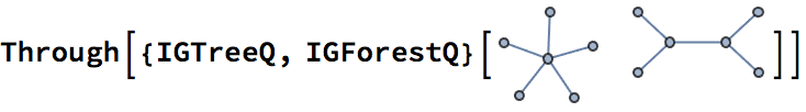
{False, True}
By convention, the null graph is not a tree, but it is a forest.
{IGTreeQ[IGEmptyGraph[0]], IGForestQ[IGEmptyGraph[0]]}{False, True}
Use the second argument to test for forests of out-trees or in-trees. By default, directed graphs are checked to be out-forests.
g = IGShorthand["1->2<-3, 4<-5->6"]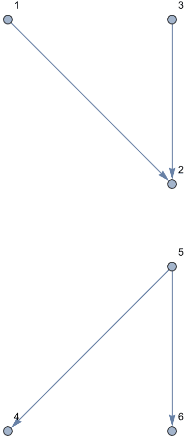
{IGForestQ[g], IGForestQ[g, "Out"], IGForestQ[g, "In"],
IGForestQ[g, "All"]}{False, False, False, True}
?IGStrahlerNumber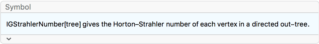
IGStrahlerNumber computes the Horton–Strahler index of
each vertex in a rooted tree. The tree must be directed—this is how the
root is encoded. The Horton–Strahler index of the tree itself is the
index of the root, i.e. the largest returned index. This measure is also
called stream order, as it was originally used to characterize
river networks.
tree = IGTreeGame[30, DirectedEdges -> True,
  GraphLayout -> "LayeredDigraphEmbedding"]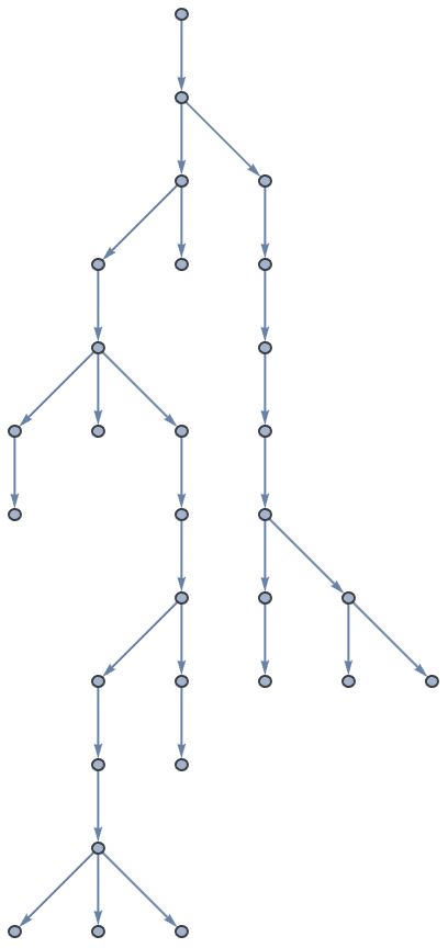
IGVertexMap[# &, VertexLabels -> IGStrahlerNumber, tree]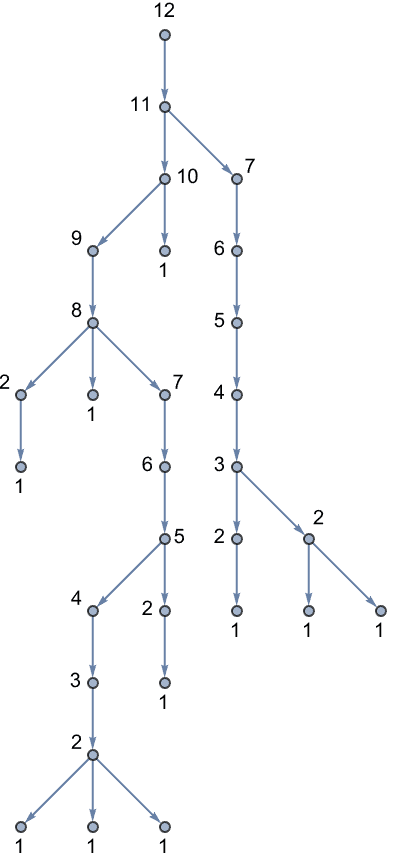
To get the Horton–Strahler number of the tree, find the maximal element.
Max@IGStrahlerNumber[tree]12
IGStrahlerNumber requires a directed (i.e. rooted) tree
as input.
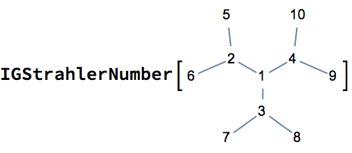
![]()
$Failed
Orient undirected trees, effectively specifying a root vertex, before
passing them to IGStrahlerNumber.
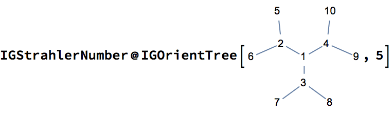
{5, 4, 3, 1, 2, 2, 1, 1, 1, 1}
?IGTreelikeComponents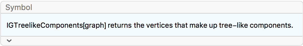
IGTreelikeComponents finds the tree-like components of an undirected graph by repeatedly identifying and removing degree-1 vertices. Vertices in the tree-like components are not part of any undirected cycle, nor are they on a path connecting vertices that belong to a cycle.
g = RandomGraph[{100, 100}];
HighlightGraph[
  g,
  IGTreelikeComponents[g]
  ] // IGLayoutFruchtermanReingold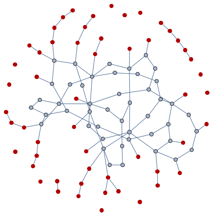
Highlight both the edges and vertices of tree-like components.
g = IGGiantComponent@RandomGraph[{50, 50}];
HighlightGraph[
 g,
 Join[
  Union @@ (IncidenceList[g, #] &) /@ IGTreelikeComponents[g],
  IGTreelikeComponents[g]
  ]
 ]
IGLayoutFruchtermanReingold[%]
Remove tree-like components.
VertexDelete[g, IGTreelikeComponents[g]]
Vertices incident to multi-edges or loop-edges are not part of tree-like components.
![]()
{1}
?IGFromPrufer
?IGToPrufer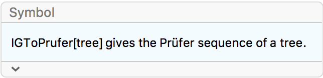
A spanning tree of a graph is a subgraph that is a tree and contains all the graph’s vertices.
?IGSpanningTree
IGSpanningTree[RandomGraph[{8, 20}], GraphStyle -> "DiagramGold"]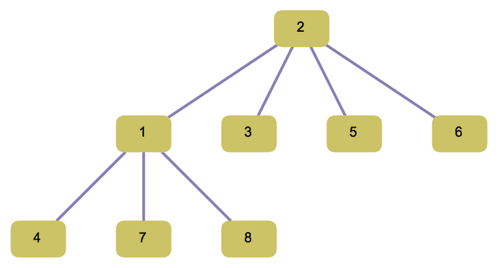
Find the shortest set of paths connecting a set of points in the plane:
pts = RandomReal[1, {10, 2}];
g = IGMeshGraph@DelaunayMesh[pts];
tree = IGSpanningTree[g, VertexCoordinates -> pts]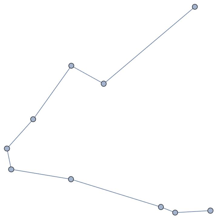
The edge weights are preserved in the result.
IGEdgeWeightedQ[tree]True
Compute the total path length.
Total@IGEdgeProp[EdgeWeight][tree]2.0021
Find a maximum spanning tree by negating the weights before running the algorithm.
IGSpanningTree[IGEdgeMap[Minus, EdgeWeight, g],
 VertexCoordinates -> pts]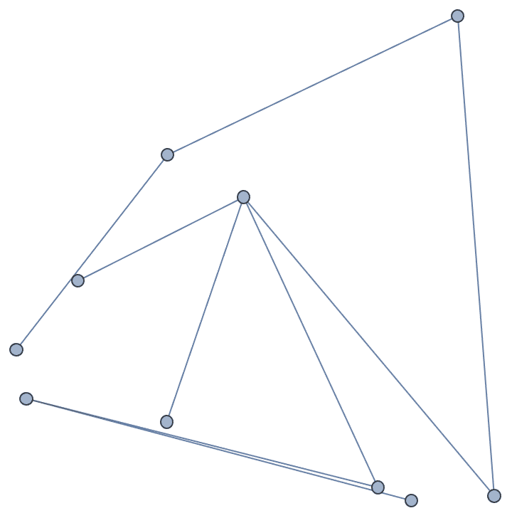
Find the minimum and maximum spanning trees of a network, using its edge betweenness as edge weights.
g = ExampleData[{"NetworkGraph", "ZacharyKarateClub"}];
HighlightGraph[
   g,
   EdgeList@
    IGSpanningTree@IGEdgeMap[#, EdgeWeight -> IGEdgeBetweenness, g],
   GraphHighlightStyle -> "Thick", ImageSize -> Small
   ] & /@ {
  Identity, (* minimum spanning tree *)
  Minus (* maximum spanning tree *)
  }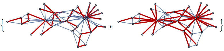
?IGRandomSpanningTree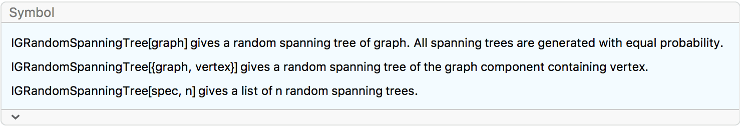
IGRandomSpanningTree samples the spanning trees (or
forests) of a graph uniformly by performing a loop-erased random walk.
Edge directions are ignored.
If a spanning forest of the entire graph is requested using
IGRandomSpanningTree[g], then the vertex names and ordering
are preserved. If a spanning tree of only a single component is
requested using IGRandomSpanningTree[{g, v}], then this is
not the case.
Highlight a few random spanning trees of the Petersen graph.
g = PetersenGraph[];
HighlightGraph[g, #, GraphHighlightStyle -> "Thick"] & /@
 IGRandomSpanningTree[g, 9]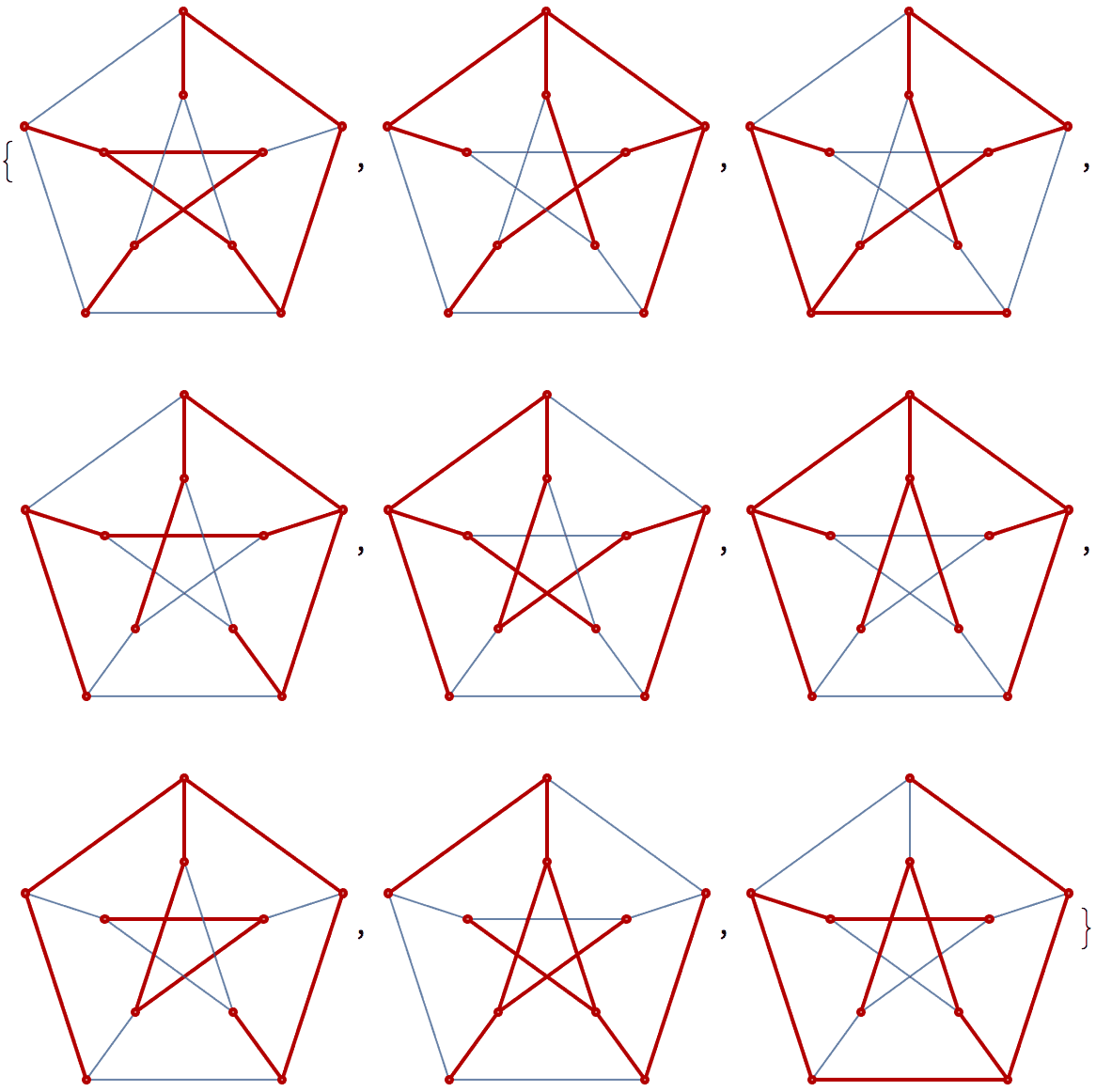
If the input is a multi-graph, each edge will be considered
separately for the purpose of spanning tree calculations. Thus the
following graph has not 3, but 5 different spanning trees. Two pairs of
these are indistinguishable based on their adjacency matrix due to the
indistinguishability of the two parallel 1 <-> 2
edges. However, since all 5 spanning trees are generated with equal
probability, two of the 3 adjacency matrices will appear twice as
frequently as the third one.
g = IGShorthand["1-2-3-1,1-2", MultiEdges -> True, ImageSize -> Small]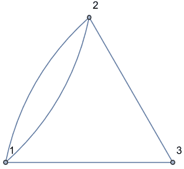
IGRandomSpanningTree[g, 10000] // CountsBy[AdjacencyMatrix] //
KeySort // KeyMap[MatrixForm]![]()
Edge directions are ignored for the purpose of spanning tree calculation. Thus the result may not be an out-tree.
IGRandomSpanningTree@WheelGraph[11, DirectedEdges -> True]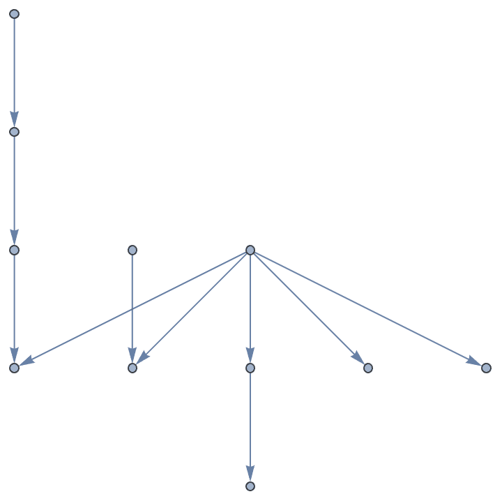
Create mazes by taking random spanning trees of grid graphs.
g = GridGraph[{10, 10}, GraphStyle -> "Web"];
HighlightGraph[g, IGRandomSpanningTree[g],
 GraphHighlightStyle -> "DehighlightHide"]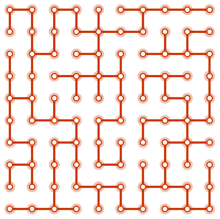
g = GridGraph[{6, 6, 6}, VertexCoordinates -> Tuples[Range[6], {3}]];
HighlightGraph[g, IGRandomSpanningTree[g],
 GraphHighlightStyle -> "DehighlightHide"]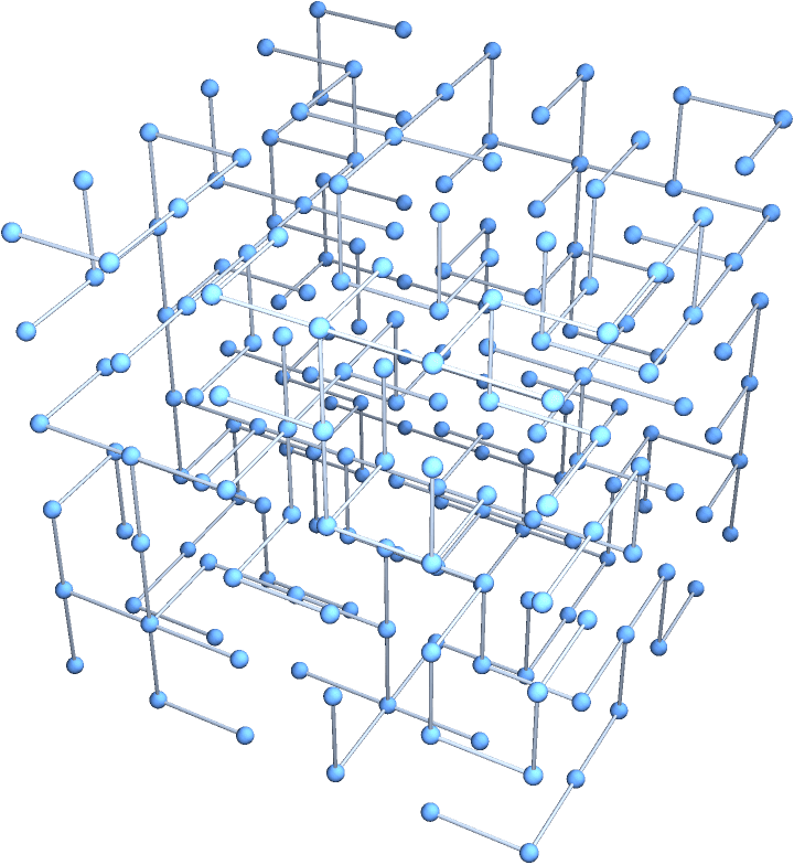
Generate a random spanning tree of the component containing vertex
8.
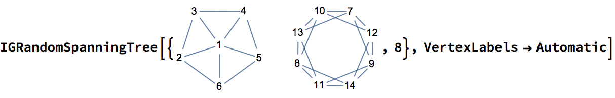
![]()
?IGSpanningTreeCount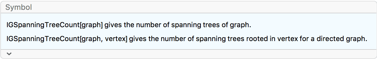
IGSpanningTreeCount computes the number of spanning
trees of a graph using Kirchhoff’s theorem. Multigraphs and directed
graphs are supported.
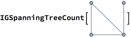
3
The number of spanning trees of a directed graph, rooted in any vertex.
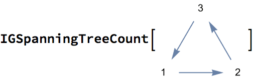
3
The number of spanning trees rooted in vertex 1.
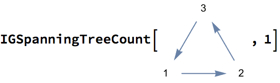
1
IGSpanningTreeCount[PetersenGraph[]]2000
IGSpanningTreeCount works on large graphs.
g = HypercubeGraph[6]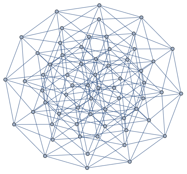
IGSpanningTreeCount[g]1657509127047778993870601546036901052416000000
Edge multiplicities are taken into account. Thus the following graph has not 3, but 5 different spanning trees.
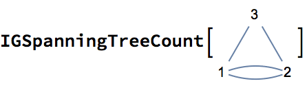
5
In a directed graph, a vertex \(d\) is said to dominate a vertex \(v\) if every path from the root to \(v\) passes through \(d\). We say that \(d\) is an immediate dominator of \(v\) if it does not dominate any other dominator of \(v\).
A dominator tree of a graph consists of the same vertices as the graph, and the children of a vertex are those other vertices which it immediately dominates.
?IGDominatorTree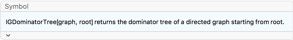
Find the dominator tree of a directed graph.
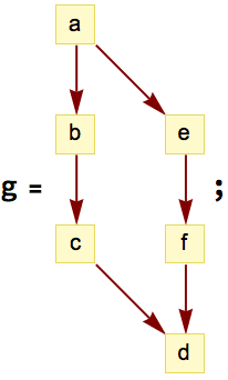
IGDominatorTree[g, "a", GraphStyle -> "VintageDiagram"]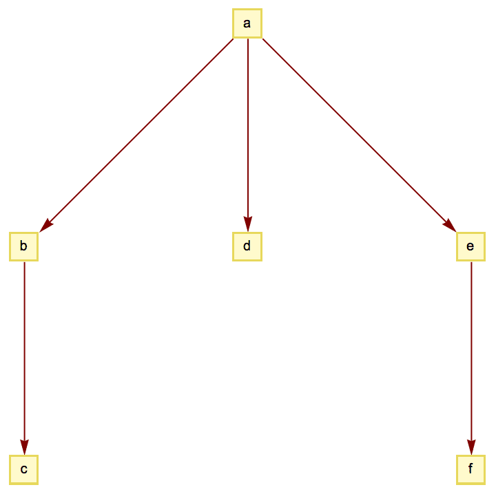
Vertices that cannot be reached from the specified root are left isolated in the returned graph.
IGDominatorTree[g, "b", GraphStyle -> "VintageDiagram"]![]()
IGDominatorTree accepts all standard Graph
options.
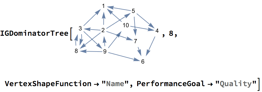
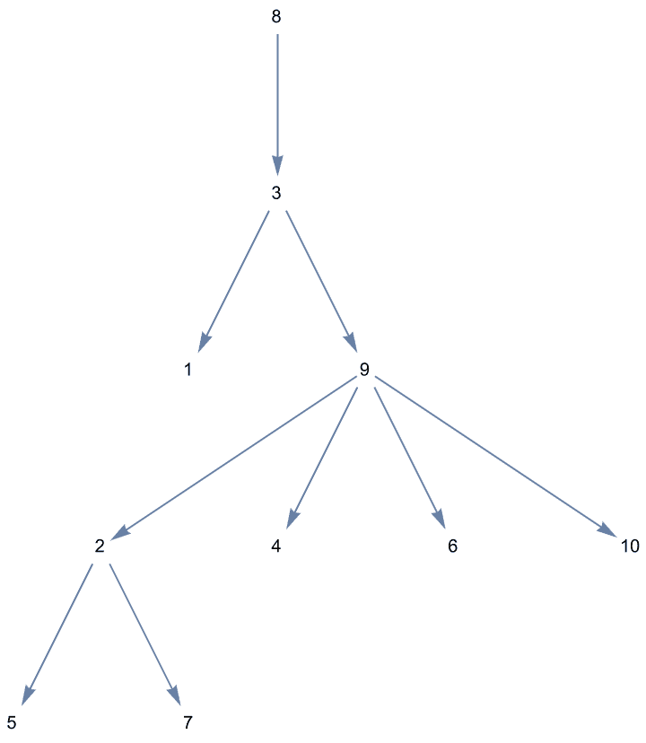
?IGImmediateDominators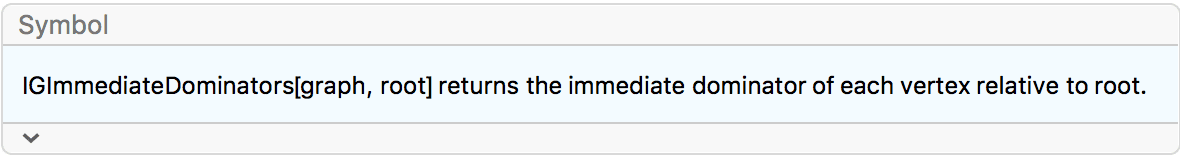
Directly find the immediate dominators of vertices in a graph.
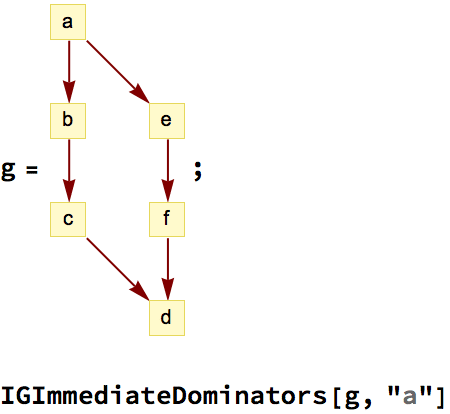
<|"b" -> "a", "c" -> "b", "d" -> "a", "e" -> "a", "f" -> "e"|>
The immediate dominator of a vertex is its parent in the dominator tree.
tree = IGDominatorTree[g, "a", VertexLabels -> Automatic]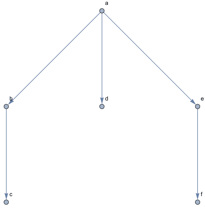
IGAdjacencyList[tree, "In"]<|"a" -> {}, "b" -> {"a"}, "c" -> {"b"}, "d" -> {"a"}, "e" -> {"a"}, "f" -> {"e"}|>
Neither the root, nor vertices unreachable from the root are included in the keys of the returned association.
IGImmediateDominators[g, "b"]<|"c" -> "b", "d" -> "c"|>
?IGCoreness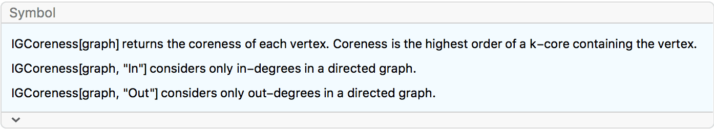
A \(k\)-core of a graph is a maximal subgraph in which each vertex has degree at least \(k\). The coreness of a vertex is the highest order of \(k\)-cores that contain it.
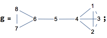
IGCoreness[g]{3, 3, 3, 3, 2, 2, 2, 2}
{KCoreComponents[g, 2], KCoreComponents[g, 3]}{{{1, 2, 3, 4, 6, 7, 8, 5}}, {{1, 2, 3, 4}}}
By default, edge directions are ignored, and multi-edges are considered.
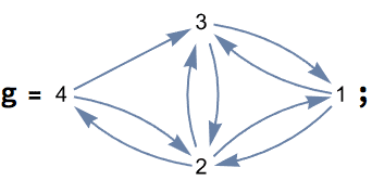
IGCoreness[g]{4, 4, 4, 3}
Use the second argument to consider only in- or out-degrees.
IGCoreness[g, "In"]{2, 2, 2, 1}
IGCoreness[g, "Out"]{2, 2, 2, 2}
A matching of a graph is a subset of its edges that share no vertices between them.
?IGMaximumMatching
A matching of a graph is also known as an independent edge set.
IGMaximumMatching ignores edge directions and edge
weights.
g = RandomGraph[{10, 20}];IGMaximumMatching[g]{7 <-> 10, 6 <-> 8, 3 <-> 9, 2 <-> 5, 1 <-> 4}
HighlightGraph[g, IGMaximumMatching[g],
 GraphHighlightStyle -> "Thick"]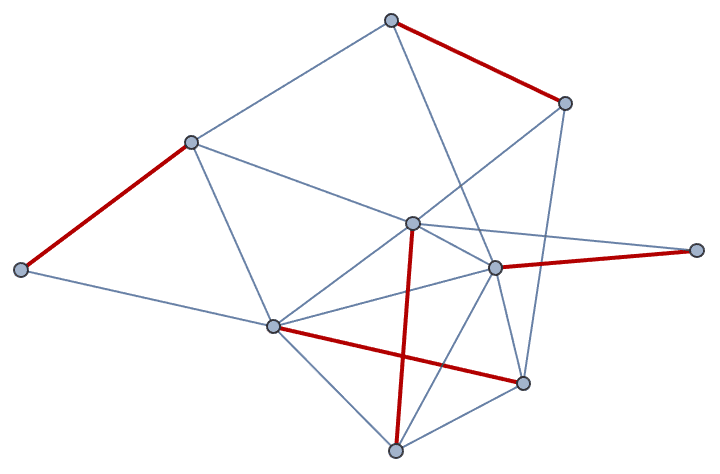
?IGMatchingNumber
The matching number of a graph is the size of its maximum matchings.
?IGUnfoldTree
IGUnfoldTree creates a tree based on the breadth-first
traversal of a graph. Each time a graph vertex is found, a new tree
vertex is created.
Available options:
DirectedEdges -> False will ignore edge directions
in directed graphs. Otherwise, the search is done only along edge
directions.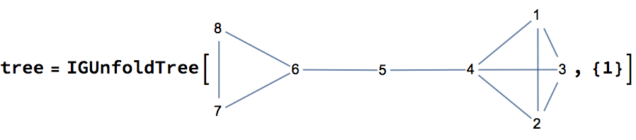
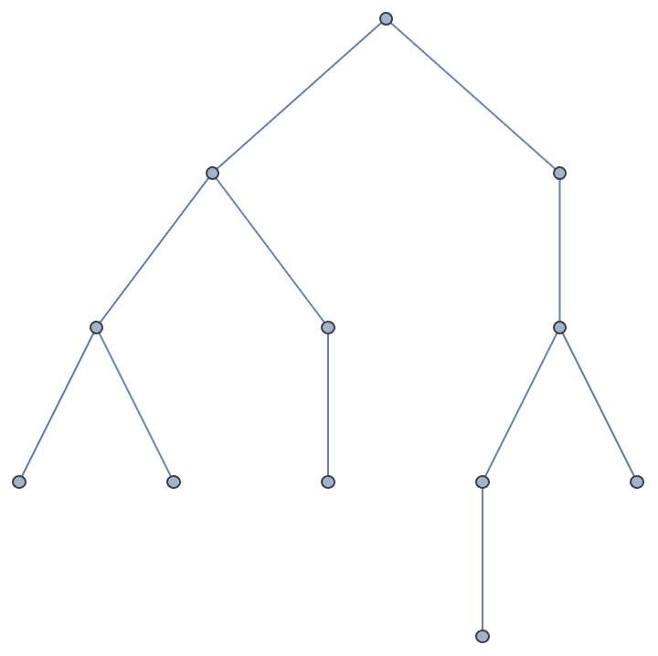
The original vertex that generates a tree node is stored in the
"OriginalVertex" property.
IGVertexProp["OriginalVertex"][tree]{1, 2, 3, 4, 6, 7, 8, 5, 3, 4, 4, 8}
We can label the tree nodes with the name of the original vertex
either using pattern matching in VertexLabels along with
PropertyValue …
IGLayoutReingoldTilford[
 tree,
 "RootVertices" -> {1},
 VertexLabels -> (v_ :> PropertyValue[{tree, v}, "OriginalVertex"])
 ]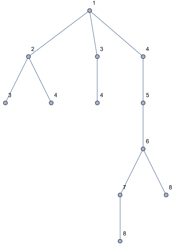
… or using IGVertexMap.
IGLayoutReingoldTilford[tree, "RootVertices" -> {1}] //
 IGVertexMap[# &, VertexLabels -> IGVertexProp["OriginalVertex"]]
In directed graphs, the search is done along edge directions. It may be necessary to give multiple starting roots to fully unfold a weakly connected (or unconnected) graph.
IGUnfoldTree[Graph[{1 -> 2, 2 -> 3}], {2, 1}] //
 IGVertexMap[# &, VertexLabels -> IGVertexProp["OriginalVertex"]]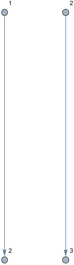
Use DirectedEdges -> False to ignore edge directions
during the search. Edge directions are still preserved in the
result.
IGUnfoldTree[Graph[{1 -> 2, 2 -> 3}], {2}, DirectedEdges -> False] //
IGVertexMap[# &, VertexLabels -> IGVertexProp["OriginalVertex"]]![]()
?IGNullGraphQ
IGNullGraphQ returns True only for the null
graph, i.e. the graph that has no vertices.
IGNullGraphQ[IGEmptyGraph[]]True
For graphs that have vertices, but no edges, it returns
False.
IGNullGraphQ[IGEmptyGraph[5]]False
In contrast, the built-in EmptyGraphQ tests if there are
no edges:
EmptyGraphQ[IGEmptyGraph[5]]True
?IGCompleteQ
IGCompleteQ tests if a graph is complete, i.e. if all
pairs of vertices are connected.
IGCompleteQ@IGCompleteGraph[10]True
IGCompleteQ@IGCompleteGraph[5, DirectedEdges -> True]True
IGCompleteQ ignores self-loops and multi-edges.
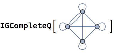
True
Check if each connected component of a graph is a clique.
g = GraphData[{8, 911}]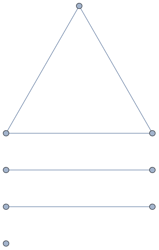
AllTrue[ConnectedGraphComponents[g], IGCompleteQ]True
The null graph is considered complete.
IGCompleteQ@IGEmptyGraph[]True
?IGCactusQ
IGCactusQ tests if a graph is a cactus. A cactus graph
is a connected undirected graph in which any two simple cycles share at
most one vertex. Equivalently, a cactus is a connected graph in which
every edge belongs to at most one simple cycle.
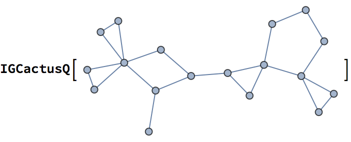
True
IGCactusQ[GridGraph[{2, 3}]]False
IGCactusQ supports multigraphs and ignores
self-loops.
![]()
{True, False}
The null graph is not considered to be a cactus, but the singleton graph is.
IGCactusQ /@ {IGEmptyGraph[0], IGEmptyGraph[1]}{False, True}
Currently, IGCactusQ does not support directed
graphs.
IGCactusQ[Graph[{1 -> 2}]]![]()
$Failed
IGraph/M’s motif-related functions count the number of times each possible connectivity pattern of \(k\) vertices (i.e. induced subgraph of size \(k\)) occurs in a graph. The patterns are called motifs. As of IGraph/M 0.6, size 3 and 4 motifs are supported in directed graphs and size 3 to 6 in undirected graphs. Only (weakly) connected subgraphs are considered.
To count larger induced subgraphs, see
IGLADSubisomorphismCount. To identify where a subgraph
occurs, see IGLADFindSubisomorphisms.
To count non-connected size-3 subgraphs, use
IGTriadCensus.
igraph’s motif functions use the RAND-ESU algorithm, which is able to
uniformly sample a random subset of motifs (connected subgraphs), and
can thus estimate motif counts even in very large graphs. See the
description of IGMotifs for an example.
?IGMotifs
IGMotifs counts how many times each motif (i.e. induced
subgraph) of the given size occurs in the graph. For subgraphs that are
not weakly connected, Indeterminate is returned.
Available options are:
DirectedEdges -> False treats the graph as
undirected and DirectedEdges -> True treats the graph as
directed. The default is DirectedEdges -> Automatic,
which respects the directedness of the graph.Motifs are returned by their IGIsoclass, i.e. the same
order as listed in IGData.
mot3 = Graph[#, ImageSize -> 36, VertexSize -> 0.1] & /@
IGData[{"AllDirectedGraphs", 3}]![]()
Let us count size-3 motifs in the following graph, and summarize them
a table. For non-weakly-connected subgraphs, Indeterminate
is returned.
g = RandomGraph[{10, 40}, DirectedEdges -> True]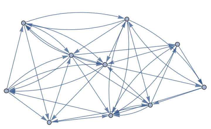
Grid[{mot3, IGMotifs[g, 3]}\[Transpose], Frame -> All]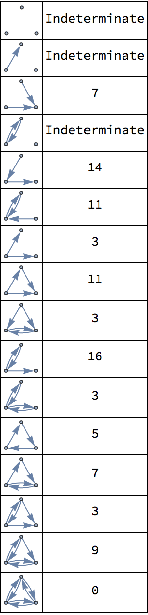
Empty graphs are treated as undirected by default. To treat them as
directed, use DirectedEdges -> True. The result will be
different as the number of non-isomorphic graphs on \(k\) vertices is not the same in the
directed and undirected cases.
IGMotifs[IGEmptyGraph[5], 3, DirectedEdges -> #] & /@ {Automatic,
True, False}{{Indeterminate, Indeterminate, 0, 0}, {Indeterminate, Indeterminate, 0, Indeterminate, 0, 0, 0, 0, 0, 0, 0, 0, 0, 0, 0, 0}, {Indeterminate, Indeterminate, 0, 0}}
Let us find the size-4 motifs that stand out in the E. coli metabolic network by comparing the motif counts to that of a rewired graph:
g = ExampleData[{"NetworkGraph", "MetabolicNetworkEscherichiaColi"}];rg = IGRewire[g, 50000];![]()
{Indeterminate, Indeterminate, Indeterminate, 1.30949, Indeterminate, \
Indeterminate, Indeterminate, 1.31896, 0.353667, Indeterminate, \
Indeterminate, Indeterminate, 0.578637, 0.58617, 0., Indeterminate, \
0.016559, 0., 0., 4.94656, 0., 0., Indeterminate, Indeterminate, \
1.29702, 0.346928, 0.165433, Indeterminate, Indeterminate, 0.674934, \
0., 0.0190229, 0., Indeterminate, Indeterminate, 0., 0., 0., 0., \
Indeterminate, 0.28928, 0.708281, 0., 0.300212, 0., 0.188359, \
0.0603697, 0., 0., 0., 0., 0., 1.37343, 0., 0.0753138, 0., 0., 0., \
0., 0., 0., 0., Indeterminate, 0., 0., 0., 31.1911, 0., 0.21875, 0., \
0., 0., 0., 0.186047, 0., 0., 1.25741, 0., 0., 0., 0., 0., 0., 0., \
0., 0., 0., 0., 0., 0., 0., Indeterminate, 0.341903, 0.129316, \
1.38161, 0., 0.0207404, 0., 0.245275, 0., 0.046376, 0., 0., 0., 0., \
0., 0., 0., 0., 0., 0.589124, 0., 0.275862, 0., 0., 0., 0., 0., 0., \
0., Indeterminate, 0.429719, 0., 0., 0., 2.11212, 0., 0., 44.6957, \
0., 0.557143, 0., 0., 0., 0., 0., 0., 0., 0., 0., 0., 0., 0., 0., 0., \
0., 2.22222, 0., 0., 0., 0., 0., 0., 0., 0., 0., 0., 0., 0., \
0.0769231, 0., 0., 0., 0., 0., 0., 0., 0., 0., 0., 0., 0., 0., 0., \
0., 0., 0., 0., 0., 0., 0., 0., 0., 0., 0., 0., 0., 0., 0., 0., 0., \
0., 0., 0., 0., 0., 0., 0., 0., 0., 0., 0., 0., Indeterminate, 0., \
0., 0., 0., Indeterminate, 0., 0., 0., 0., 0., 0., Indeterminate, 0., \
Indeterminate}
largeRatios = Select[ratios, # > 5 &]{31.1911, 44.6957}
There are two motifs that are more than 30 times more common in the metabolic network than in the rewired graph.
Extract[IGData[{"AllDirectedGraphs", 4}],
   FirstPosition[ratios, #]] & /@ largeRatios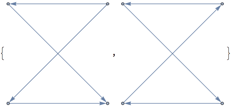
The Davidson–Harel algorithm attempts to reduce edge crossings and can draw these subgraphs in a clearer way:
IGLayoutDavidsonHarel /@ %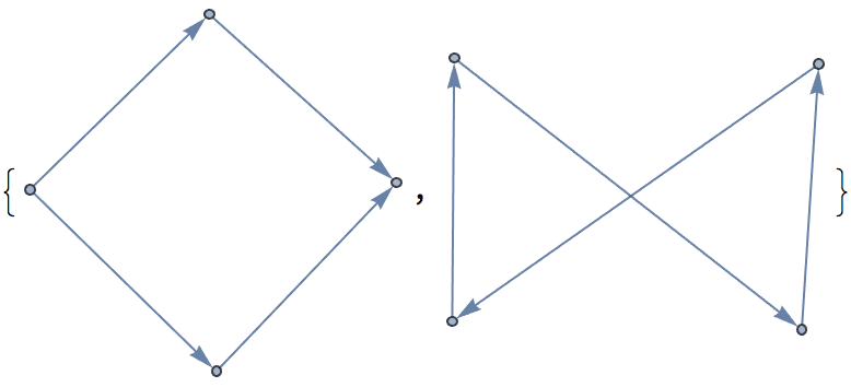
IGMotifs uses the RAND-ESU algorithm which can uniformly
sample a random subset of motifs, and thus estimate motif counts even in
very large graphs. To enable random sampling, set a cutoff probability
![]() for
stopping the search at each level of the ESU tree. The length of the
cutoff probability vector,
for
stopping the search at each level of the ESU tree. The length of the
cutoff probability vector, n, must be the same as the motif
size. The number of sampled motifs is, on average, a fraction
![]() of
the total number.
of
the total number.
bigG = ExampleData[{"NetworkGraph", "WorldWideWeb"}];
{VertexCount[bigG], EdgeCount[bigG]}{325729, 1497134}
Sample a fraction \(0.1^3=0.001\) of all motifs.
IGMotifs[bigG, 3, 1 - 0.1 {1, 1, 1}] // AbsoluteTiming{0.502014, {Indeterminate, Indeterminate, 34953, Indeterminate, 1549, 1646, 27314, 378, 291, 681, 3917, 2, 49, 171, 71, 7010}}
Sample 12.5% of motifs, i.e. a fraction of \(0.5^3\).
IGMotifs[bigG, 3, 1 - 0.5 {1, 1, 1}] // AbsoluteTiming{9.29356, {Indeterminate, Indeterminate, 36350526, Indeterminate, 299314, 530929, 5424564, 67262, 34048, 166963, 516326, 1730, 4461, 204276, 12329, 800823}}
?IGMotifsVertexParticipation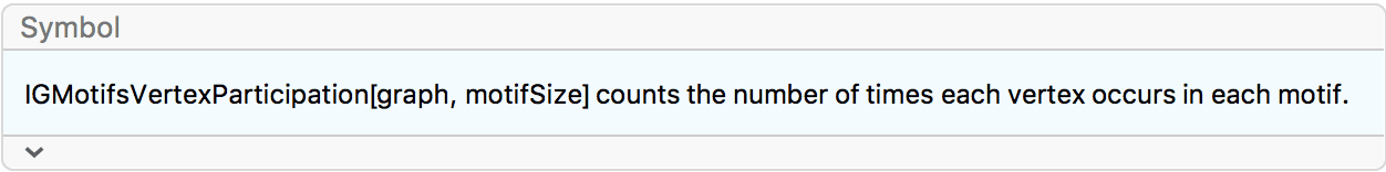
IGMotifsVertexParticipation counts how many times each
vertex participates in each motif. For each vertex, the result is
returned in the same format as with IGMotifs.
Available options are:
DirectedEdges -> False treats the graph as
undirected and DirectedEdges -> True treats the graph as
directed. The default is DirectedEdges -> Automatic,
which respects the directedness of the graph.Count how many times each vertex appears in each 3-motif in a directed graph.
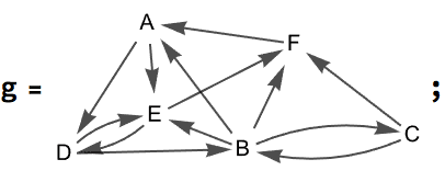
mot = IGMotifsVertexParticipation[g, 3]<|"A" -> {Indeterminate, Indeterminate, 0, Indeterminate, 2, 0, 0, 2, 1, 1, 0, 2, 0, 0, 0, 0}, "B" -> {Indeterminate, Indeterminate, 0, Indeterminate, 1, 1, 0, 3, 0, 2, 0, 1, 1, 1, 0, 0}, "C" -> {Indeterminate, Indeterminate, 1, Indeterminate, 1, 1, 0, 0, 0, 2, 0, 0, 0, 1, 0, 0}, "D" -> {Indeterminate, Indeterminate, 0, Indeterminate, 2, 1, 0, 0, 1, 1, 0, 1, 1, 0, 0, 0}, "E" -> {Indeterminate, Indeterminate, 1, Indeterminate, 0, 0, 0, 2, 1, 2, 0, 1, 1, 0, 0, 0}, "F" -> {Indeterminate, Indeterminate, 1, Indeterminate, 3, 0, 0, 2, 0, 1, 0, 1, 0, 1, 0, 0}|>
The sum of the participation counts in 3-motifs is 3 times the total motif counts of the graph.
Total[mot] === 3 IGMotifs[g, 3]True
?IGMotifsTotalCount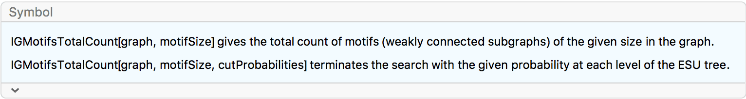
?IGMotifsTotalCountEstimate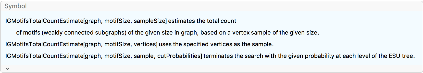
IGMotifsTotalCount[graph, motifSize] counts the number
of weakly connected subgraphs of the given size in a graph. All subgraph
sizes greater than 2 are supported.
IGMotifsTotalCountEstimate[graph, motifSize, sampleSize]
estimates the total number of motifs by taking a random subset of
vertices of the specified size, and counting motifs in which these
vertices participate. The total number is estimated as
motifCount*vertexCount/sampleSize.
IGMotifsTotalCountEstimate[graph, motifSize, vertices] uses
the specified vertices as the sample.
Let us create a graph.
g = RandomGraph[{20, 50}];The number of size-4 subgraphs it has is:
Binomial[VertexCount[g], 4]4845
However, only a small fraction of these is connected:
IGMotifsTotalCount[g, 4]779
IGMotifsTotalCount is effectively equivalent to (but
much faster than) the following:
Count[Subsets[VertexList[g], {4}],
 subset_ /; WeaklyConnectedGraphQ@Subgraph[g, subset]]
779
Estimate the count of connected subgraphs by subsampling: at each level of the ESU tree, continue only with probability 0.9.
IGMotifsTotalCount[g, 4, 1 - 0.9 {1, 1, 1, 1}]/0.9^4833.714
Estimate the count of connected subgraphs by considering a random subset of 15 vertices (out of a total of 20).
IGMotifsTotalCountEstimate[g, 4, 15]994
Use the first 15 vertices tot estimate the count.
IGMotifsTotalCountEstimate[g, 4, Range[15]]1038
?IGTriadCensus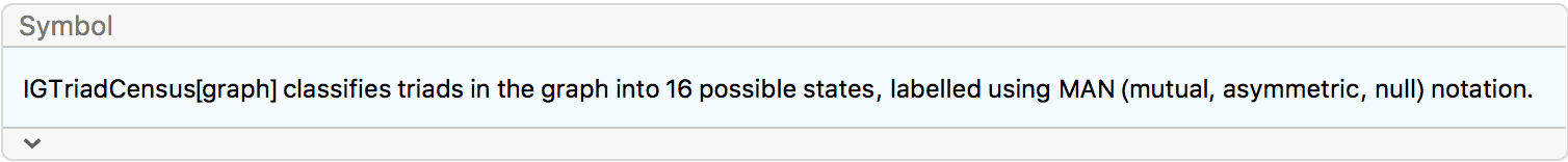
?IGDyadCensus
See IGData["MANTriadLabels"] for the mapping between MAN
labels and graphs.
IGTriadCensus[g] does not return triad counts in the
same order as IGMotifs[g, 3], i.e. ordered according to the
triads’ IGIsoclass[]. To get the result ordered by
isoclass, use
Lookup[IGTriadCensus[g], Keys@IGData["MANTriadLabels"]]IGData["MANTriadLabels"] are ordered according to
isoclass.
net = ExampleData[{"NetworkGraph",
"MetabolicNetworkActinobacillusActinomycetemcomitans"}];IGDyadCensus[net]<|"Mutual" -> 32, "Asymmetric" -> 2304, "Null" -> 490192|>
IGTriadCensus[net]<|"003" -> 160429739, "012" -> 2191799, "102" -> 30579, "021D" -> 11774, "021U" -> 10566, "021C" -> 22853, "111D" -> 496, "111U" -> 583, "030T" -> 0, "030C" -> 0, "201" -> 27, "120D" -> 0, "120U" -> 0, "120C" -> 0, "210" -> 0, "300" -> 0|>
?IGTriangles
Highlight all triangles in a graph.
g = RandomGraph[{8, 16}, VertexSize -> Large];HighlightGraph[g, Subgraph[g, #], ImageSize -> Tiny,
GraphHighlightStyle -> "Thick"] & /@ IGTriangles[g]
?IGAdjacentTriangleCount
Label a graph’s vertices based on the number of adjacent triangles.
RandomGraph[{8, 16}, VertexSize -> Large] //
 IGVertexMap[Placed[#, Center] &,
  VertexLabels -> IGAdjacentTriangleCount]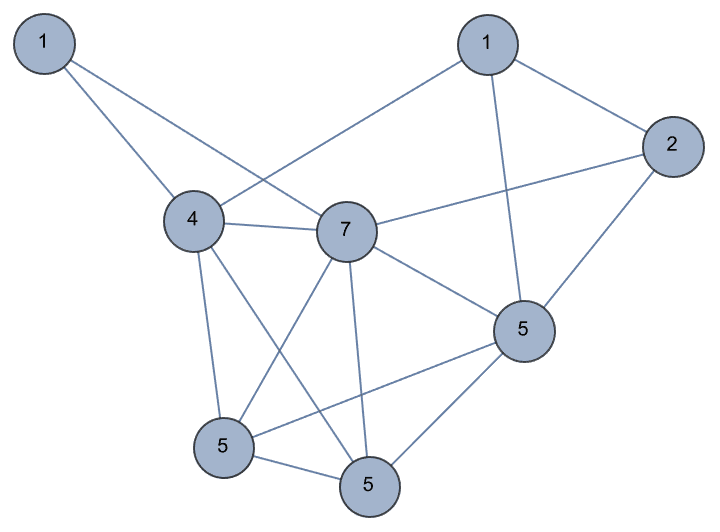
Triangle-free graphs do not have any fully connected subgraphs of size 3. Equivalently, they do not have any cliques (other than 2-cliques, which are edges).
?IGTriangleFreeQ
Mycielski graphs are triangle-free.
IGTriangleFreeQ@GraphData[{"Mycielski", 10}]True
igraph implements three isomorphism testing algorithms: BLISS, VF2 and LAD. These support slightly different functionality.
Naming: Most of IGraph/M’s isomorphism related
functions include the name of the algorithm as a prefix,
e.g. IGBlissIsomorphicQ. Functions named as
…GetIsomorphism will find a single isomorphism. Functions
named as …FindIsomorphisms can find multiple isomorphisms.
Both return a result in a format compatible with the built-in
FindGraphIsomorphism.
Additionally, IGIsomorphicQ[] and
IGSubisomorphicQ[] try to select the best algorithm for the
given graphs. For graphs without multi-edges, they use igraph’s default
algorithm selection. For multigraphs, they use VF2 after internally
transforming the multigraphs to edge- and vertex-coloured simple graphs,
in a manner similar to IGColoredSimpleGraph.
?IGIsomorphicQ
?IGGetIsomorphism
IGIsomorphicQ decides if two graphs are isomorphic.
IGIsomorphicQ[IGShorthand["a-b-c-a-d"], IGShorthand["1-2,3-4-2-3"]]True
IGIsomorphicQ supports multigraphs.
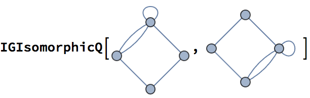
True
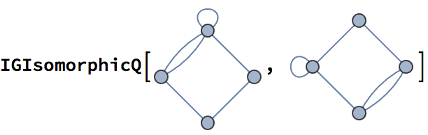
False
Get a specific mapping between the vertices of the graphs.
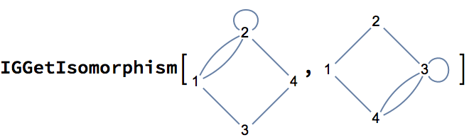
{<|1 -> 4, 2 -> 3, 3 -> 1, 4 -> 2|>}
When the graphs are not isomorphic, an empty list is returned.
IGGetIsomorphism[CycleGraph[4], IGCompleteGraph[4]]{}
?IGSubisomorphicQ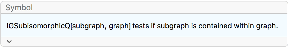
?IGGetSubisomorphism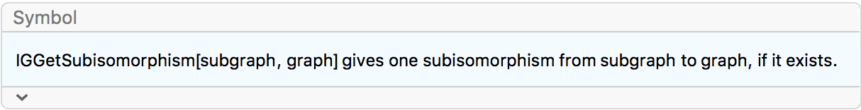
IGSubisomorphicQ decides if a subgraph is part of a
larger graph.
A dodecahedral graph does not contain a [1, 2, 3]
symmetric tree.
target = GraphData["DodecahedralGraph"];
pattern = IGSymmetricTree[{1, 2, 3}];IGSubisomorphicQ[pattern, target]False
It does contain a [3, 2, 1] tree.
pattern = IGSymmetricTree[{3, 2, 1}];
IGSubisomorphicQ[pattern, target]
True
Let us retrieve a specific mapping …
{iso} = IGGetSubisomorphism[pattern, target]{<|1 -> 1, 2 -> 14, 3 -> 15, 4 -> 16, 5 -> 3, 6 -> 9, 7 -> 4, 8 -> 10, 9 -> 7, 10 -> 8, 11 -> 19, 12 -> 17, 13 -> 20, 14 -> 18, 15 -> 11, 16 -> 12|>}
… and highlight it.
HighlightGraph[target, VertexReplace[pattern, Normal[iso]],
 GraphHighlightStyle -> "Thick"
 ]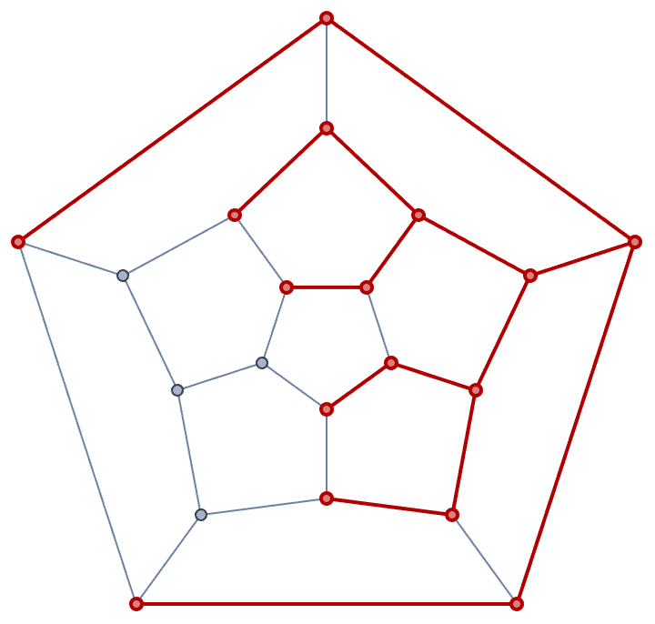
IGSubisomorphicQ supports multigraphs.
![]()
True
![]()
{<|"a" -> 1, "b" -> 2|>}
![]()
True
![]()
False
The Bliss library was developed by Tommi Junttila and Petteri Kaski. It is capable of canonical labelling of directed or undirected vertex coloured graphs.
Bliss generally outperforms Mathematica’s built-in isomorphisms functions (including finding and counting automorphisms) as of Mathematica 12.1. However, this advantage will only be apparent for large and difficult graphs. For small ones the overhead of having to copy the graph and convert it to igraph’s internal format is much larger than the actual computation time.
?IGBliss*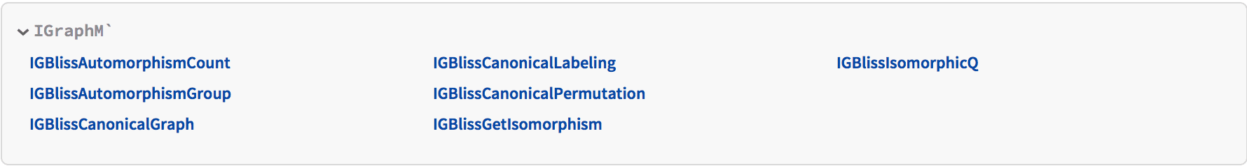
All Bliss functions take a "SplittingHeuristics" option,
which can influence the performance of the method. Possible values
are:
"First" – First non-unit cell. Very fast but may
result in large search spaces on difficult graphs. Use for large but
easy graphs.
"FirstSmallest" – First smallest non-unit cell.
Fast, should usually produce smaller search spaces than
"First".
"FirstLargest" – First largest non-unit cell. Fast,
should usually produce smaller search spaces than
"First".
"FirstMaximallyConnected" – First maximally
non-trivially connected non-unit cell. Not so fast, should usually
produce smaller search spaces than "First",
"FirstSmallest" and "FirstLargest".
"FirstSmallestMaximallyConnected" – First smallest
maximally non-trivially connected non-unit cell. Not so fast, should
usually produce smaller search spaces than "First",
"FirstSmallest" and "FirstLargest".
"FirstLargestMaximallyConnected" – First largest
maximally non-trivially connected non-unit cell. Not so fast, should
usually produce smaller search spaces than "First",
"FirstSmallest" and "FirstLargest".
The default setting is "FirstLargest", which performs
well on average on sparse graphs.
Note: The result of the
IGBlissCanonicalLabeling,
IGBlissCanonicalPermutation and
IGBlissanonicalGraph functions depend on the choice of
"SplittingHeuristics". See the Bliss
documentation for more information.
Let us take the cuboctahedral graph from GraphData …
g1 = GraphData["CuboctahedralGraph"]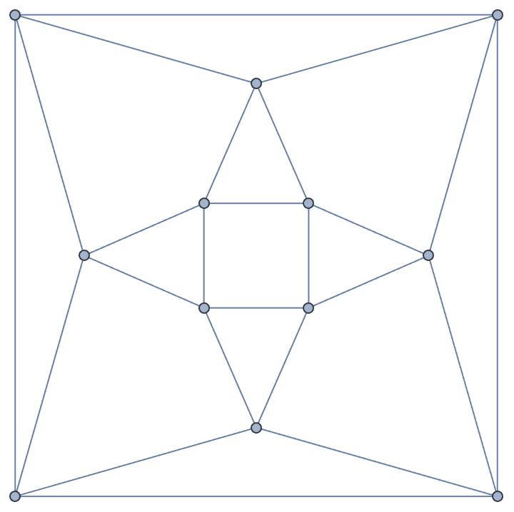
… and also generate it based on its LCF notation.
g2 = IGLCF[{4, 2}, 6]
The two graphs are isomorphic:
IGBlissIsomorphicQ[g1, g2]True
One particular mapping between them is the following:
IGBlissGetIsomorphism[g1, g2]{<|1 -> 1, 2 -> 2, 3 -> 5, 4 -> 12, 5 -> 9, 6 -> 4, 7 -> 10, 8 -> 3, 9 -> 6, 10 -> 11, 11 -> 8, 12 -> 7|>}
How many mappings are there in total? The same number as the number of automorphisms of either graph.
IGBlissAutomorphismCount[g1]48
Bliss cannot generate all 48 of these mappings directly. We can either use VF2 for this …
IGVF2FindIsomorphisms[g1, g2] // Length48
… or we can use the automorphism group computed by the
IGBlissAutomorphismGroup function.
group = IGBlissAutomorphismGroup[g1]PermutationGroup[{Cycles[{{2, 3}, {4, 5}, {8, 9}, {10, 11}}], Cycles[{{2, 4}, {3, 5}, {6, 7}, {8, 10}, {9, 11}}], Cycles[{{1, 2}, {3, 6}, {5, 8}, {7, 10}, {11, 12}}]}]
GroupOrder[group]48
Ask for all 48 vertex permutations that create isomorphic graphs:
PermutationReplace[VertexList[g1], group]{{1, 2, 3, 4, 5, 6, 7, 8, 9, 10, 11, 12}, {1, 3, 2, 5, 4, 6, 7, 9, 8, 11, 10, 12}, {1, 4, 5, 2, 3, 7, 6, 10, 11, 8, 9, 12}, {1, 5, 4, 3, 2, 7, 6, 11, 10, 9, 8, 12}, {2, 1, 6, 4, 8, 3, 10, 5, 9, 7, 12, 11}, {2, 4, 8, 1, 6, 10, 3, 7, 12, 5, 9, 11}, {2, 6, 1, 8, 4, 3, 10, 9, 5, 12, 7, 11}, {2, 8, 4, 6, 1, 10, 3, 12, 7, 9, 5, 11}, {3, 1, 6, 5, 9, 2, 11, 4, 8, 7, 12, 10}, {3, 5, 9, 1, 6, 11, 2, 7, 12, 4, 8, 10}, {3, 6, 1, 9, 5, 2, 11, 8, 4, 12, 7, 10}, {3, 9, 5, 6, 1, 11, 2, 12, 7, 8, 4, 10}, {4, 1, 7, 2, 10, 5, 8, 3, 11, 6, 12, 9}, {4, 2, 10, 1, 7, 8, 5, 6, 12, 3, 11, 9}, {4, 7, 1, 10, 2, 5, 8, 11, 3, 12, 6, 9}, {4, 10, 2, 7, 1, 8, 5, 12, 6, 11, 3, 9}, {5, 1, 7, 3, 11, 4, 9, 2, 10, 6, 12, 8}, {5, 3, 11, 1, 7, 9, 4, 6, 12, 2, 10, 8}, {5, 7, 1, 11, 3, 4, 9, 10, 2, 12, 6, 8}, {5, 11, 3, 7, 1, 9, 4, 12, 6, 10, 2, 8}, {6, 2, 3, 8, 9, 1, 12, 4, 5, 10, 11, 7}, {6, 3, 2, 9, 8, 1, 12, 5, 4, 11, 10, 7}, {6, 8, 9, 2, 3, 12, 1, 10, 11, 4, 5, 7}, {6, 9, 8, 3, 2, 12, 1, 11, 10, 5, 4, 7}, {7, 4, 5, 10, 11, 1, 12, 2, 3, 8, 9, 6}, {7, 5, 4, 11, 10, 1, 12, 3, 2, 9, 8, 6}, {7, 10, 11, 4, 5, 12, 1, 8, 9, 2, 3, 6}, {7, 11, 10, 5, 4, 12, 1, 9, 8, 3, 2, 6}, {8, 2, 10, 6, 12, 4, 9, 1, 7, 3, 11, 5}, {8, 6, 12, 2, 10, 9, 4, 3, 11, 1, 7, 5}, {8, 10, 2, 12, 6, 4, 9, 7, 1, 11, 3, 5}, {8, 12, 6, 10, 2, 9, 4, 11, 3, 7, 1, 5}, {9, 3, 11, 6, 12, 5, 8, 1, 7, 2, 10, 4}, {9, 6, 12, 3, 11, 8, 5, 2, 10, 1, 7, 4}, {9, 11, 3, 12, 6, 5, 8, 7, 1, 10, 2, 4}, {9, 12, 6, 11, 3, 8, 5, 10, 2, 7, 1, 4}, {10, 4, 8, 7, 12, 2, 11, 1, 6, 5, 9, 3}, {10, 7, 12, 4, 8, 11, 2, 5, 9, 1, 6, 3}, {10, 8, 4, 12, 7, 2, 11, 6, 1, 9, 5, 3}, {10, 12, 7, 8, 4, 11, 2, 9, 5, 6, 1, 3}, {11, 5, 9, 7, 12, 3, 10, 1, 6, 4, 8, 2}, {11, 7, 12, 5, 9, 10, 3, 4, 8, 1, 6, 2}, {11, 9, 5, 12, 7, 3, 10, 6, 1, 8, 4, 2}, {11, 12, 7, 9, 5, 10, 3, 8, 4, 6, 1, 2}, {12, 8, 9, 10, 11, 6, 7, 2, 3, 4, 5, 1}, {12, 9, 8, 11, 10, 6, 7, 3, 2, 5, 4, 1}, {12, 10, 11, 8, 9, 7, 6, 4, 5, 2, 3, 1}, {12, 11, 10, 9, 8, 7, 6, 5, 4, 3, 2, 1}}
Permuting the adjacency matrix with any of these leaves it invariant.
perms = PermutationList[#, VertexCount[g1]] & /@
   GroupElements[group];
Equal @@ (AdjacencyMatrix[g1][[#, #]] & /@ perms)
True
Bliss works by computing a canonical labelling of vertices. Then isomorphism can be tested for by comparing the canonically relabelled graphs.
IGBlissCanonicalGraph[g1] === IGBlissCanonicalGraph[g2]True
IGBlissCanonicalGraph returns graphs in a consistent
format so that two graphs are isomorphic if and only if their canonical
graphs will compare equal with ===. Note that in
Mathematica, graphs may not always compare equal even if they
have the same vertex and edge lists.
The corresponding permutation and labelling are
IGBlissCanonicalPermutation[g1]{12, 11, 9, 10, 8, 7, 6, 5, 3, 4, 2, 1}
IGBlissCanonicalLabeling[g1]<|1 -> 12, 2 -> 11, 3 -> 9, 4 -> 10, 5 -> 8, 6 -> 7, 7 -> 6, 8 -> 5, 9 -> 3, 10 -> 4, 11 -> 2, 12 -> 1|>
Notice that the canonical labelling is simply
AssociationThread[VertexList[g1], IGBlissCanonicalPermutation[g1]]<|1 -> 12, 2 -> 11, 3 -> 9, 4 -> 10, 5 -> 8, 6 -> 7, 7 -> 6, 8 -> 5, 9 -> 3, 10 -> 4, 11 -> 2, 12 -> 1|>
Also notice that it is a mapping from g1 to
IGBlissCanonicalGraph[g1]:
MemberQ[
 IGVF2FindIsomorphisms[g1, IGBlissCanonicalGraph[g1]],
 IGBlissCanonicalLabeling[g1]
 ]
True
The canonical graph returned by IGBlissCanonicalGraph
always has vertices labelled by the integers 1, 2, … It can
also be used to filter duplicates from a list of graphs
For example, let us generate all possible adjacency matrices of 3-vertex simple directed graphs.
(* fills nondiagonal entries of n by n matrix from vector *)
toMat[vec_, n_] :=
 SparseArray@
  Partition[Flatten@Riffle[Partition[vec, n], 0, {1, -1, 2}], n]
There are 2^(3 2) = 2^6 = 64 such matrices.
graphs =
  AdjacencyGraph[toMat[#, 3], DirectedEdges -> True] & /@
   IntegerDigits[Range[2^6] - 1, 2, 6];
But only 16 of them correspond to non-isomorphic graphs
DeleteDuplicatesBy[graphs, IGBlissCanonicalGraph] // Length16
When IGBlissCanonicalGraph is given a vertex coloured
graph, it will encode the colours into a vertex property named
"Color". This allows distinguishing between graphs whose
canonical graphs are identical in structure, but differ in
colouring.
Take for example the following coloured graphs:
g = Graph[{1 <-> 2, 2 <-> 3},
   VertexSize -> Large, GraphStyle -> "BasicBlack"];
colg1 = Graph[g,
   Properties -> {1 -> {"color" -> 1}, 2 -> {"color" -> 3},
     3 -> {"color" -> 2}}];
colg2 = Graph[g,
   Properties -> {1 -> {"color" -> 1}, 2 -> {"color" -> 3},
     3 -> {"color" -> 1}}];
Visualize them for clarity:
IGVertexMap[ColorData[97],
VertexStyle -> IGVertexProp["color"]] /@ {colg1, colg2}![]()
The vertex and edge lists of their canonical graphs are identical:
cang1 = IGBlissCanonicalGraph[{colg1, "VertexColors" -> "color"}];
cang2 = IGBlissCanonicalGraph[{colg2, "VertexColors" -> "color"}];
VertexList /@ {cang1, cang2}
EdgeList /@ {cang1, cang2}{{1, 2, 3}, {1, 2, 3}}
{{1 <-> 3,
 2 <-> 3}, {1 <-> 3,
 2 <-> 3}}
But they differ in colouring, and therefore do not compare equal:
IGVertexPropertyList[cang1]{"Color", VertexCoordinates, VertexShape, VertexShapeFunction, \ VertexSize, VertexStyle}
IGVertexProp["Color"] /@ {cang1, cang2}{{1, 2, 3}, {1, 1, 3}}
cang1 === cang2False
The performance of Bliss functions may depend significantly on the choice of splitting heuristics.
g = LineGraph@GraphData[{"Hadamard", {24, 6}}];
timings = {#,
     First@Timing@
       IGBlissAutomorphismGroup[g, "SplittingHeuristics" -> #]} & /@
   {"First", "FirstSmallest", "FirstLargest",
    "FirstMaximallyConnected", "FirstSmallestMaximallyConnected",
    "FirstLargestMaximallyConnected"};
TableForm[timings,
 TableHeadings -> {None, {"Splitting heuristics", "Timing (s)"}}]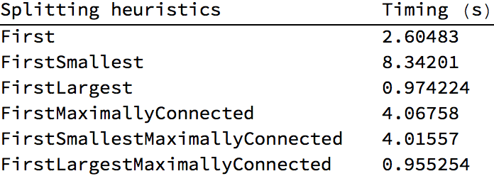
Let us visualize the vertex equivalence classes induced by a graph’s automorphism group. Two vertices are considered equivalent if there is an automorphism that maps one into the other.
With[{g = GraphData[{"Mycielski", 4}]},
 HighlightGraph[g, GroupOrbits@IGBlissAutomorphismGroup[g],
  VertexSize -> Large, GraphStyle -> "BasicBlack"]
 ]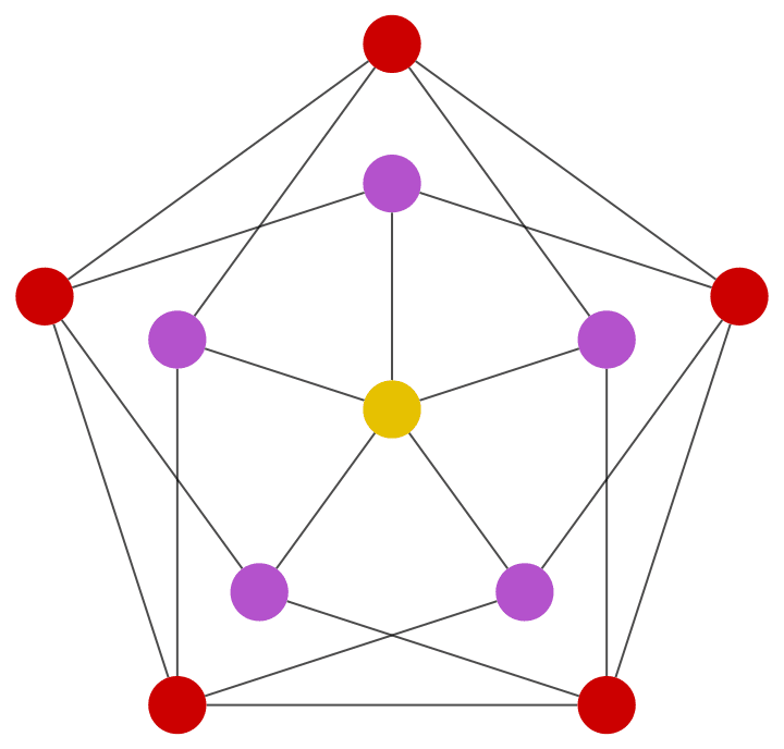
Visualize the edge equivalence classes of a polyhedron, induced by its skeleton’s automorphism group.
mesh = PolyhedronData["TruncatedOctahedron", "BoundaryMeshRegion"]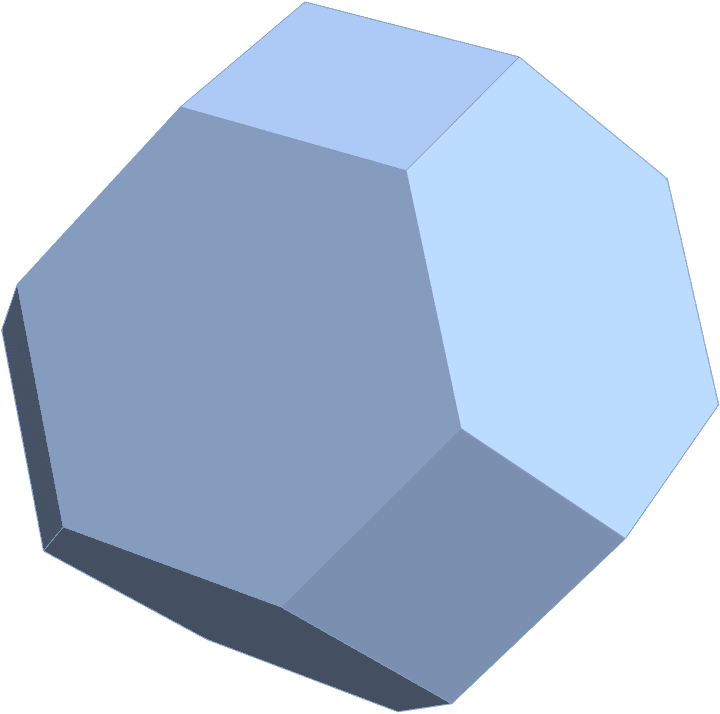
With[{g = IGMeshGraph[mesh, VertexStyle -> Black]},
 HighlightGraph[g,
  EdgeList[g][[#]] & /@
   GroupOrbits@IGBlissAutomorphismGroup@LineGraph[g]
  ]
 ]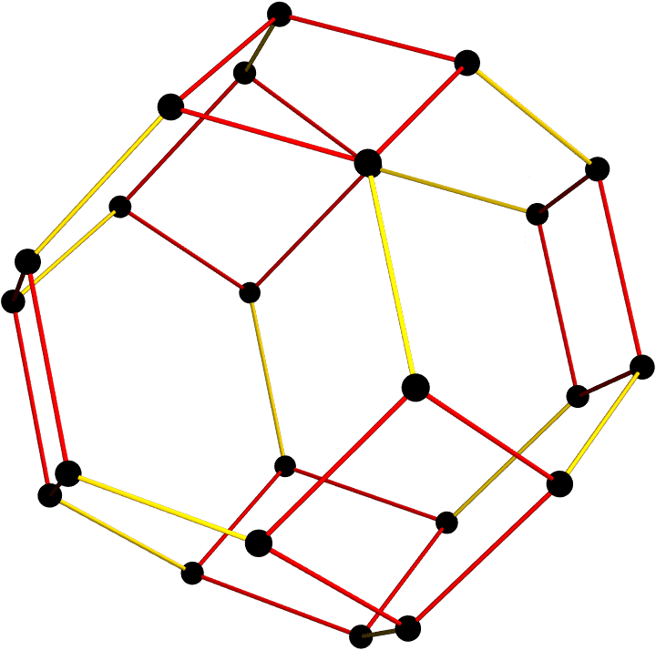
?IGVF2*
VF2 supports vertex coloured and edge coloured graphs. A colour
specification consists of one or more of the "VertexColors"
and "EdgeColors" options. Allowed formats for these options
are a list of integers, an association assigning integers to the
vertices/edges, or None. When using associations, it is not
necessarily to specify a colour for each vertex/edge. The omitted ones
are assumed to have colour 0.
The VF2 algorithm only supports simple graphs.
The following graph has two automorphisms: {1, 2} and
{2, 1}.
g = Graph[{1 <-> 2}];
IGVF2IsomorphismCount[g, g]
2
If we colour one of the vertices, the permutation {2, 1}
becomes forbidden, so only one automorphism remains.
IGVF2IsomorphismCount[{g, "VertexColors" -> {1, 2}}, {g,
  "VertexColors" -> {1, 2}}]
1
Multigraphs are not directly supported for isomorphism checking, but we can map the multigraph isomorphism problem into an edge-coloured graph isomorphism one by designating the multiplicity of each edge as its colour.
g1 = EdgeAdd[PathGraph[Range[5], VertexLabels -> "Name"],
2 <-> 3]![]()
g2 = EdgeAdd[PathGraph[Range[5], VertexLabels -> "Name"],
4 <-> 3]![]()
IGVF2IsomorphicQ[g1, g2]![]()
$Failed
Since g1 and g2 are undirected, we need to
bring their edges into a sorted canonical form before counting them.
This ensures that 4 <-> 3 and
3 <-> 4 are treated as the same edge.
colors1 = Counts[Sort /@ EdgeList[g1]]<|1 <-> 2 -> 1, 2 <-> 3 -> 2, 3 <-> 4 -> 1, 4 <-> 5 -> 1|>
colors2 = Counts[Sort /@ EdgeList[g2]]<|1 <-> 2 -> 1, 2 <-> 3 -> 1, 3 <-> 4 -> 2, 4 <-> 5 -> 1|>
IGVF2IsomorphicQ[{Graph@Keys[colors1],
  "EdgeColors" -> colors1}, {Graph@Keys[colors2],
  "EdgeColors" -> colors2}]
True
IGIsomorphicQ and IGSubisomorphicQ check
multigraph isomorphism in a similar way, based on edge colouring.
The LAD library was developed by Christine Solnon. It is capable of finding subgraphs in a larger graph.
The LAD algorithm does not support multi-edges.
?IGLAD*
With the "Induced" -> True option LAD will search for
induced subgraphs.
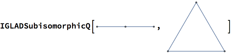
True
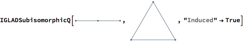
False
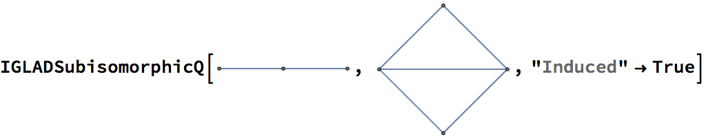
True
Highlight subgraphs in a grid graph.
g = GridGraph[{3, 3}];
HighlightGraph[g, Subgraph[g, #], GraphHighlightStyle -> "Thick"] & /@
  Union[Sort@*Values /@
   IGLADFindSubisomorphisms[GridGraph[{2, 2}], g]]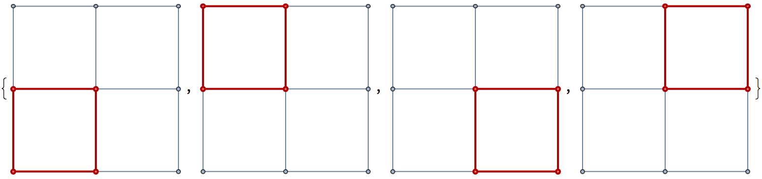
Count how many times each vertex of a graph appears at the apex of the following subgraph (motif):
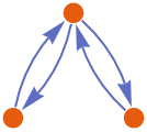
Generate a directed random graph to do the counting in.
g = RandomGraph[{20, 120}, DirectedEdges -> True]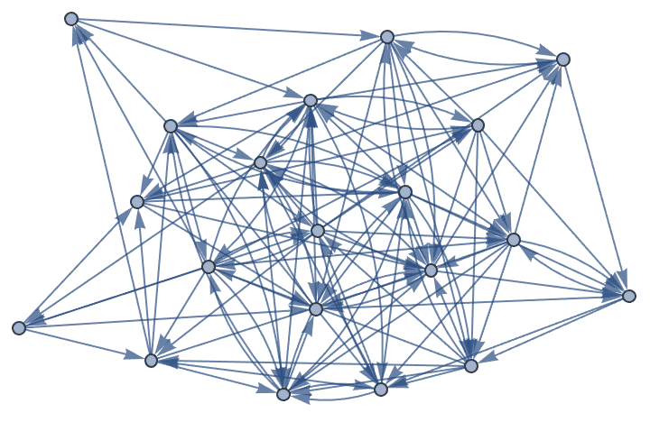
IGShorthand provides a concise way to input this
subgraph.
motif = IGShorthand["2<->1<->3"]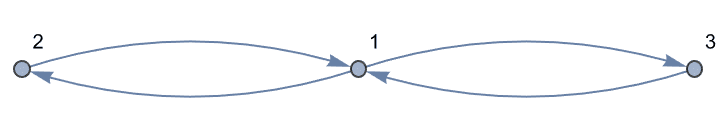
This motif has a two-fold symmetry, as revealed by its automorphism group. We divide the final counts by two.
Counts@Lookup[
   IGLADFindSubisomorphisms[motif, g, "Induced" -> True],
   1
]/IGBlissAutomorphismCount[motif]<|13 -> 2, 18 -> 2, 20 -> 4, 12 -> 1, 16 -> 1|>
Check that a graph is claw-free.
clawFreeQ[graph_?UndirectedGraphQ] :=
 Not@IGLADSubisomorphicQ[
   StarGraph[4], (* claw graph *)
   graph,
   "Induced" -> True
   ]
clawFreeQ /@ {GraphData["DodecahedralGraph"],
GraphData["TruncatedPrismGraph"]}{False, True}
All three included isomorphism algorithms support vertex coloured
graphs, and VF2 supports edge coloured graphs as well. A coloured graph
is specified as
{g, "VertexColors" -> …, "EdgeColors" -> …}, where
both vertex and edge colour specifications are optional. Colours are
represented by integers and may be specified in one of the following
ways:
A list of integers, given in the same order as
VertexList[g] (or EdgeList[g] if specifying
edge colours).
{Graph[{a, b}, {a <-> b}], "VertexColors" -> {1, 2}}.
An association assigning integers to vertices (or edges).
Vertices (or edges) not present in the association are assumed to have
colour 0.
{Graph[{a <-> b}], "VertexColors" -> <|a -> 1, b -> 2|>}.
The name of a a vertex (or edge) property. Vertices (or edges)
without an assigned property value are assumed to have colour
0.
{Graph[{Property[a, "color" -> 1], Property[b, "color" -> 2]}, {a <-> b}], "VertexColors" -> "color"}
"VertexColors" -> None indicates no
colouring.
Example. Define a graph along with the colours of its vertices.
g = CycleGraph[4];
vcols = <|
1 -> 1, 2 -> 1,
3 -> 2, 4 -> 2
|>;Visualize it.
Graph[g,
VertexStyle -> Normal[ColorData[24] /@ vcols],
VertexSize -> Medium, VertexLabels -> Placed["Name", Center]
]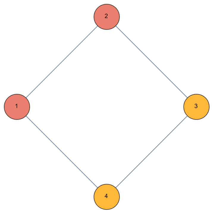
Compute its automorphism group, taking vertex colours into account.
IGBlissAutomorphismGroup[{g, "VertexColors" -> vcols}]PermutationGroup[{Cycles[{{1, 2}, {3, 4}}]}]
The functions in this section test for properties related to a graph’s automorphism group. The summary table below illustrates the functions on a set of graphs which all have different properties.
graphs = {StarGraph[4], IGSquareLattice[{2, 3}, "Periodic" -> True],
HypercubeGraph[3], GraphData[{"Rook", {4, 4}}],
GraphData["ShrikhandeGraph"], GraphData["HoltGraph"],
GraphData["Tutte12Cage"], GraphData[{"Paulus", {25, 1}}]};
functions = <|
"regular" -> IGRegularQ,
"strongly regular" -> IGStronglyRegularQ,
"distance regular" -> IGDistanceRegularQ,
"vertex transitive" -> IGVertexTransitiveQ,
"edge transitive" -> IGEdgeTransitiveQ,
"arc transitive" -> IGEdgeTransitiveQ@*DirectedGraph,
"distance transitive" -> IGDistanceTransitiveQ
|>;
TableForm[
Through[Values[functions][#]] & /@ graphs,
TableHeadings -> {Show[#, ImageSize -> 50] & /@ graphs,
Keys[functions]},
TableDirections -> Row
] // Style[#, "Text"] &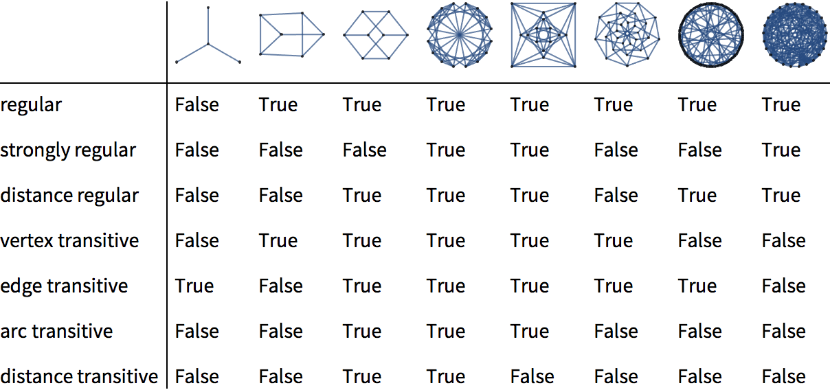
?IGRegularQ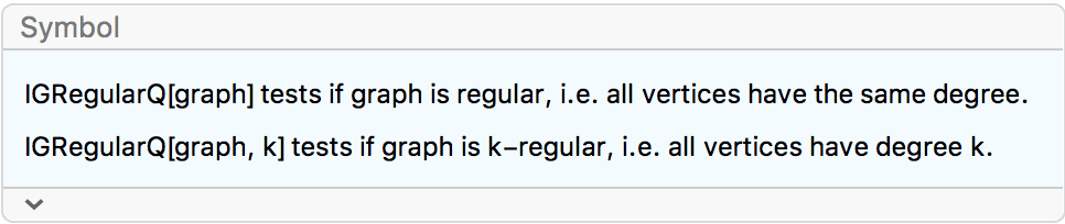
IGRegularQ checks if a graph is regular. All vertices of
a regular graph have the same degrees. In regular directed graphs, the
in- and out-degrees are also equal to each other.
IGRegularQ[IGSquareLattice[{3, 4}, "Periodic" -> True]]True
Check if a graph is \(k\)-regular for \(k=2\) and \(k=3\).
IGRegularQ[CycleGraph[10], 2]True
IGRegularQ[CycleGraph[10], 3]False
The null graph is considered 0-regular.
IGRegularQ[IGEmptyGraph[]]True
Check if a directed graph is regular.
IGRegularQ[CycleGraph[5, DirectedEdges -> True]]True
IGRegularQ considers self-loops and multi-edges when
computing vertex degrees.
![]()
True
?IGStronglyRegularQ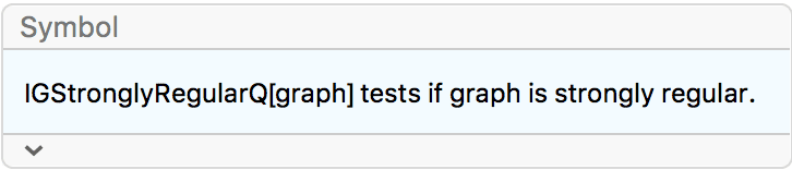
IGStronglyRegularQ checks if a graph is strongly
regular. A strongly regular graph is a regular graph where each pair of
connected vertices have the same number of common neighbours, \(\lambda\), and each pair of unconnected
vertices also have the same number of common neighbours, \(\mu\).
IGStronglyRegularQ@GraphData["ShrikhandeGraph"]True
Hypercube graphs and 3 and higher dimensions are not strongly regular, even though they are regular.
IGStronglyRegularQ /@ HypercubeGraph /@ Range[2, 4]{True, False, False}
Some authors exclude empty and complete graph from the definition, as
they satisfy these conditions trivially. IGStronglyRegularQ
returns True for these.
IGStronglyRegularQ /@ {IGEmptyGraph[5], IGCompleteGraph[6]}{True, True}
It also returns True for graphs on 0, 1 and 2
vertices.
IGStronglyRegularQ /@ IGCompleteGraph /@ Range[0, 2]{True, True, True}
Currently, IGStronglyRegularQ does not support directed
graphs.
IGStronglyRegularQ@Graph[{1 -> 2}]![]()
$Failed
?IGStronglyRegularParameters
IGStronglyRegularParameters returns the parameters \((v,k,\lambda ,\mu )\) of a strongly regular
graph. \(v\) is the number of vertices,
\(k\) the degree of the vertices, \(\lambda\) the number of common neighbours
of connected vertices and \(\mu\) the
number of common neighbours of unconnected vertices.
IGStronglyRegularParameters[PetersenGraph[]]{10, 3, 0, 1}
IGStronglyRegularParameters[CycleGraph[5]]{5, 2, 0, 1}
The parameters of a strongly regular graph satisfy the equation \((v-k-1)\mu =k(k-\lambda -1)\).
{v, k, lambda, mu} =
IGStronglyRegularParameters[GraphData[{"Paley", 101}]]{101, 50, 24, 25}
(v - k - 1) mu == k (k - lambda - 1)True
\(\lambda\) and \(\mu\) are not well-defined for empty and complete graphs, respectively. In these cases, 0 is returned.
IGStronglyRegularParameters /@ {IGEmptyGraph[5], IGCompleteGraph[6]}{{5, 0, 0, 0}, {6, 5, 4, 0}}
For non-strongly-regular graphs, {} is returned.
IGStronglyRegularParameters[HypercubeGraph[3]]{}
?IGDistanceRegularQ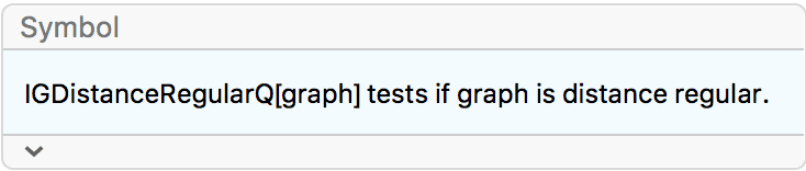
IGDistanceRegularGraph checks if a graph is distance
regular.
IGDistanceRegularQ@HypercubeGraph[5]True
IGDistanceRegularQ@IGSquareLattice[{2, 5}, "Periodic" -> True]False
A distance regular graph with a diameter of 2 is also strongly regular.
g = GraphData[{"Paley", 13}]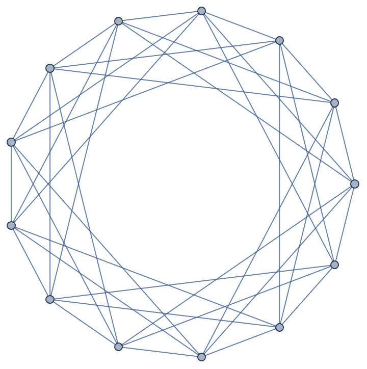
{IGDiameter[g], IGDistanceRegularQ[g], IGStronglyRegularQ[g]}{2, True, True}
The Shrikhande graph is the smallest graph that is distance regular, but not distance transitive.
Through[{IGDistanceRegularQ, IGDistanceTransitiveQ}[
GraphData["ShrikhandeGraph"]]]{True, False}
A disconnected graph is distance regular if its components are distance regular and they are co-spectral. The following graphs are co-spectral:
components = {GraphData[{"Rook", {4, 4}}],
GraphData["ShrikhandeGraph"]}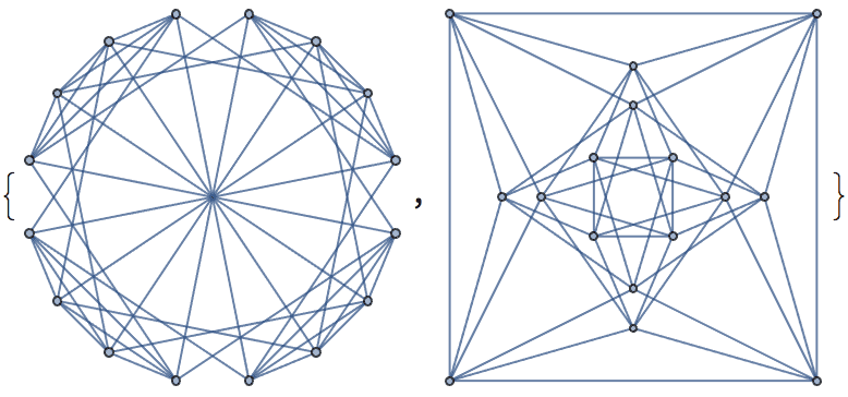
Eigenvalues /@ AdjacencyMatrix /@ components{{6, -2, -2, -2, -2, -2, -2, -2, -2, -2, 2, 2, 2, 2, 2, 2}, {6, -2, -2, -2, -2, -2, -2, -2, -2, -2, 2, 2, 2, 2, 2, 2}}
They are both distance regular with the same intersection array.
IGIntersectionArray /@ components{{{6, 3}, {1, 2}}, {{6, 3}, {1, 2}}}
Thus their disjoint union is also distance regular.
IGDistanceRegularQ@IGDisjointUnion[components]True
All distance transitive graphs are also distance regular, but the reverse is not true.
IGDistanceTransitiveQ /@ components{True, False}
IGDistanceRegularQ does not currently support directed
graphs or non-simple graphs.
IGDistanceRegularQ[Graph[{1 -> 2}]]![]()
$Failed
IGDistanceRegularQ[
Graph[{1 <-> 2, 1 <-> 2}]]![]()
$Failed
?IGIntersectionArray
IGIntersectionArray@GraphData["IcosahedralGraph"]{{5, 2, 1}, {1, 2, 5}}
IGIntersectionArray@GraphData["SuzukiGraph"]{{416, 315}, {1, 96}}
IGIntersectionArray@CycleGraph[6]{{2, 1, 1}, {1, 1, 2}}
For non-distance-regular graphs, {} is returned.
IGIntersectionArray[GridGraph[{3, 3}]]{}
IGIntersectionArray does not currently support directed
graphs.
IGIntersectionArray[Graph[{1 -> 2}]]![]()
$Failed
?IGVertexTransitiveQ
IGVertexTransitiveQ checks if a graph is vertex
transitive, i.e. if any vertex can be mapped into any other by some
automorphism of the graph.
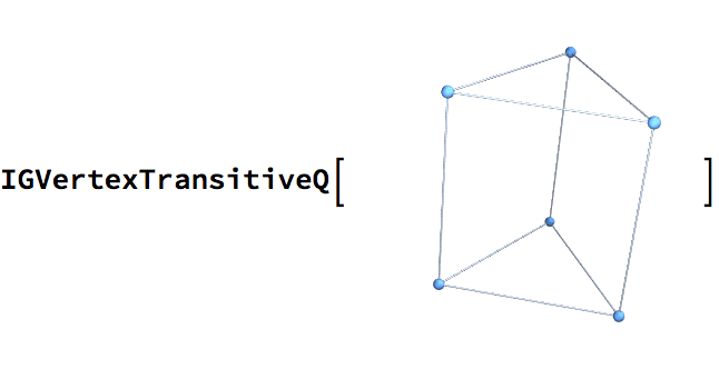
True
![]()
False
All Cayley graphs are vertex transitive.
cg = CayleyGraph@IGBlissAutomorphismGroup@IGLCF[{2, -1, 2}, 3]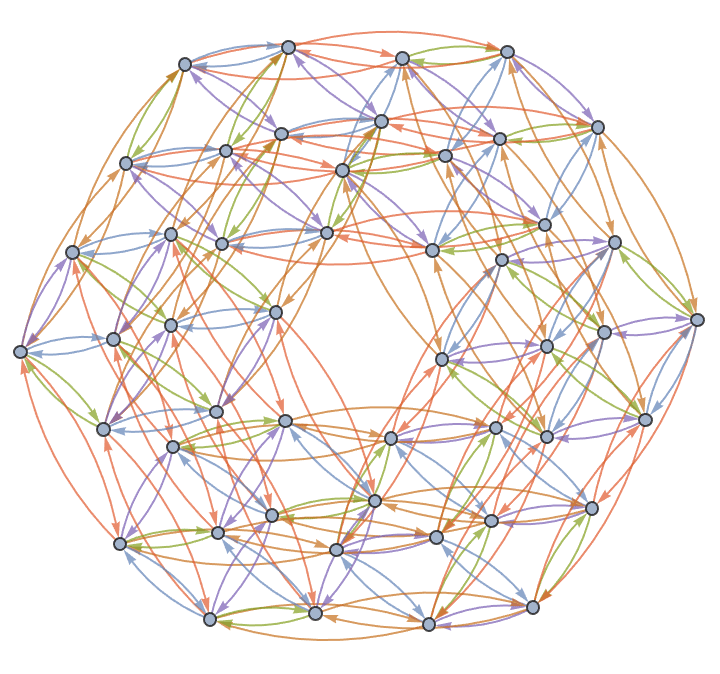
IGVertexTransitiveQ[cg]True
?IGEdgeTransitiveQ
IGEdgeTransitiveQ checks if a graph is edge transitive,
i.e. if any edge can be mapped into any other by some automorphism of
the graph.
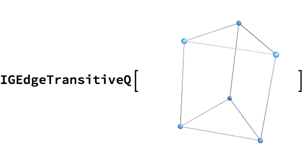
False
![]()
True
The Folkman graph is not vertex transitive but it is edge transitive.
Through[{IGVertexTransitiveQ, IGEdgeTransitiveQ}@
GraphData["FolkmanGraph"]]{False, True}
IGEdgeTransitiveQ takes into account edge
directions.
IGEdgeTransitiveQ@Graph[{1 -> 2, 2 -> 3}]False
IGEdgeTransitiveQ@Graph[{1 -> 2, 3 -> 2}]True
Arc transitivity in an undirected graph refers to edge transitivity when each undirected edge is replaced by two opposite directed edges.
arcTransitiveQ[graph_?UndirectedGraphQ] :=
IGEdgeTransitiveQ@DirectedGraph[graph]Some graphs are edge transitive, but not arc transitive.
IGEdgeTransitiveQ@GraphData[{"Bouwer", {2, 4, 15}}]True
arcTransitiveQ@GraphData[{"Bouwer", {2, 4, 15}}]False
Most graphs are edge transitive if their line graphs are vertex transitive. The exceptions are disjoint unions of the 3-star and 3-cycle. These two graphs have the same line graph, but they are not isomorphic.
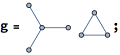
{IGEdgeTransitiveQ[g], IGVertexTransitiveQ@LineGraph[g]}{False, True}
?IGSymmetricQ
IGSymmetricQ checks if a graph is both vertex transitive
and edge transitive. Note that this property is distinct from being
arc transitive, which is the definition used for
“symmetric” by some authors.
IGSymmetricQ[GraphData["DodecahedralGraph"]]True
Make a table of symmetric graphs up to size 7:
Grid[
Table[
Graph[#, ImageSize -> 50, PlotTheme -> "Business"] & /@
Select[GraphData /@ GraphData[k], IGSymmetricQ],
{k, 1, 7}
], Frame -> All, ItemSize -> All]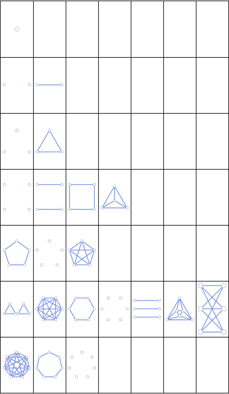
Some authors use the term symmetric graph to refer to arc
transitive graphs. Arc transitivity can be checked using
IGEdgeTransitiveQ@DirectedGraph[#] &. All
arc-transitive graphs are both vertex- and edge-transitive, but the
reverse is not true. The smallest graph that is both vertex- and
edge-transitive, but not arc-transitive, is the 27-vertex Doyle graph,
also known as the Holt graph.
doyle = GraphData["DoyleGraph"]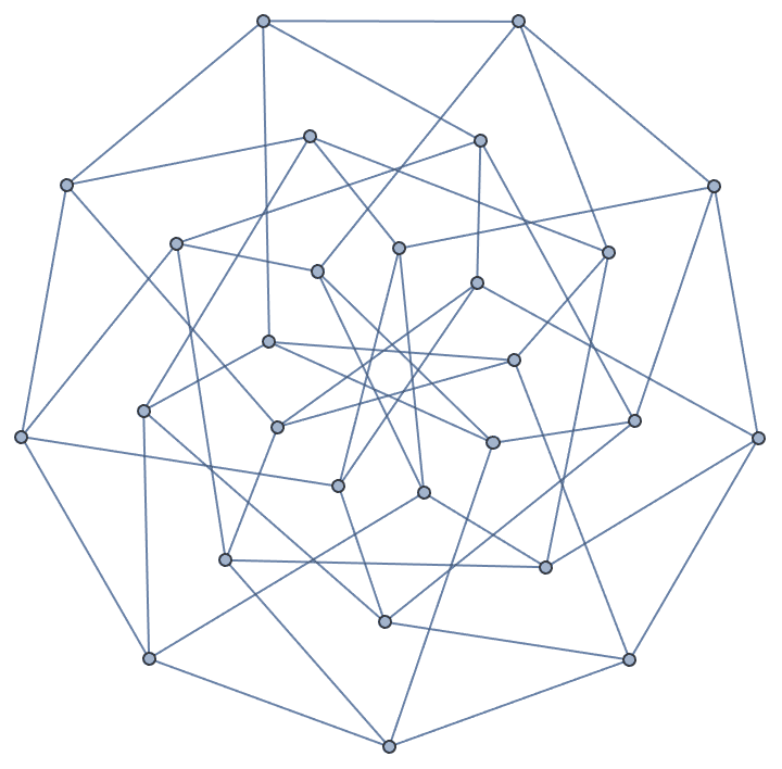
{IGVertexTransitiveQ[doyle], IGEdgeTransitiveQ[doyle]}{True, True}
IGEdgeTransitiveQ@DirectedGraph[doyle]False
?IGDistanceTransitiveQ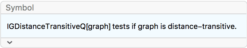
IGDistanceTransitiveQ checks if a graph is distance
transitive. In a distance transitive graph, any two ordered pairs of
vertices which are the same distance apart can be mapped into each other
by some automorphism.
All Platonic graphs are distance transitive.
IGMeshGraph@PolyhedronData[#, "BoundaryMeshRegion"] & /@
PolyhedronData["Platonic"]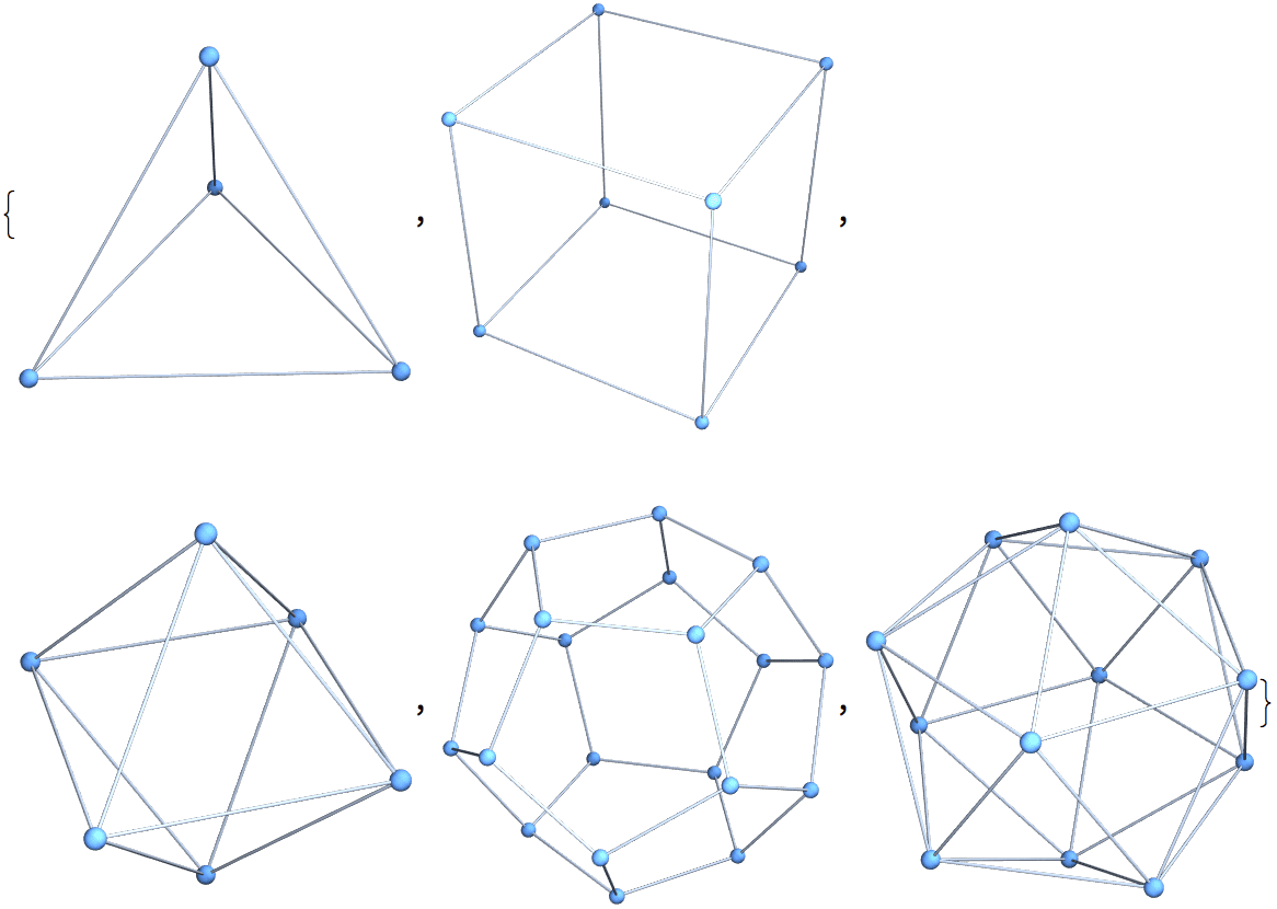
IGDistanceTransitiveQ /@ %{True, True, True, True, True}
Some graphs are symmetric, but not distance transitive.
g = GraphData[{"Circulant", {10, {1, 4}}}]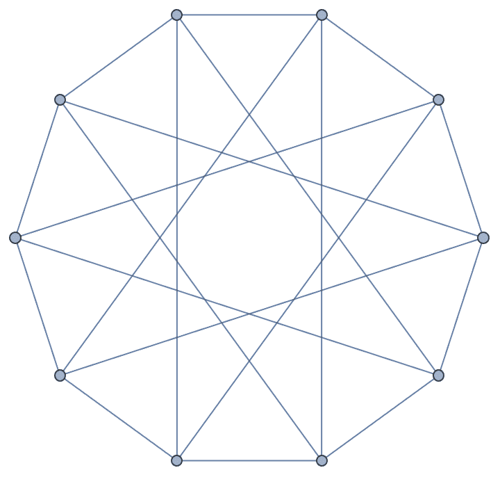
{IGSymmetricQ[g], IGDistanceTransitiveQ[g]}{True, False}
IGDistanceTransitiveQ does not exclude non-connected
graphs.
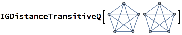
True
IGDistanceTransitiveQ works with directed graphs.
g = With[{n = 11},
RelationGraph[
MemberQ[Rest@Union@Mod[Range[n]^2, n], Mod[#1 - #2, n]] &,
Range[n] - 1]
]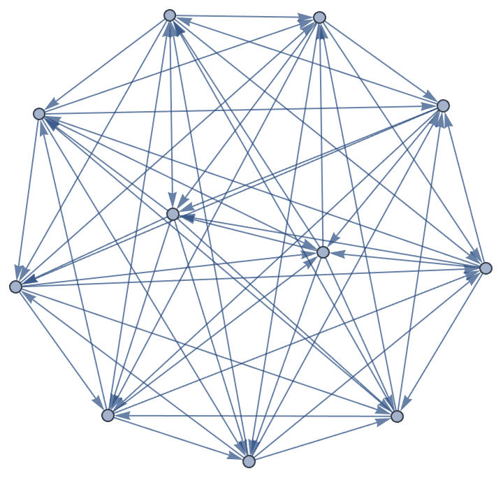
IGDistanceTransitiveQ[g]True
The following directed graph is vertex transitive, but not distance transitive.
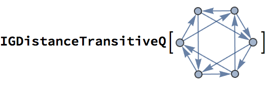
False
?IGHomeomorphicQ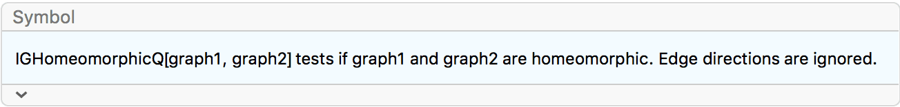
IGHomeomorphicQ tests if two graphs are homeomorphic,
i.e. whether they have the same topological structure. Two graphs \(G_1\) and \(G_2\) are homeomorphic if there is an
isomorphism from a subdivision of \(G_1\) to a subdivision of \(G_2\).
![]() is effectively implemented as
is effectively implemented as
![]() .
.
The following graphs are homeomorphic.
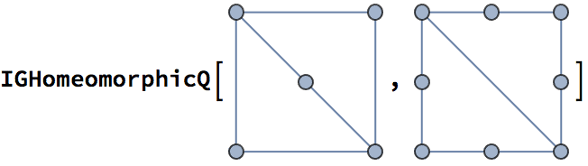
True
They smoothen to the same graph.
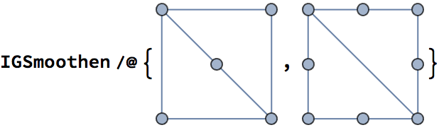
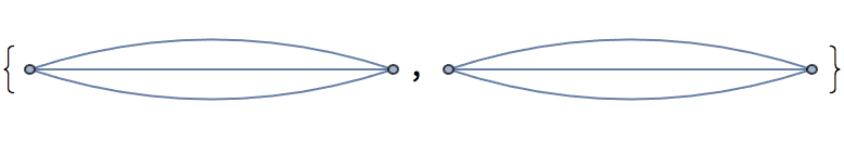
Any two cycle graphs are homeomorphic.
IGHomeomorphicQ[CycleGraph[5], CycleGraph[9]]True
A cycle and a path graph are not homeomorphic.
IGHomeomorphicQ[CycleGraph[5], PathGraph@Range[5]]False
A triangular and a square lattice on the same number of vertices are, in general, topologically different.
IGHomeomorphicQ[IGSquareLattice[{3, 3}], IGTriangularLattice[{3, 3}]]False
When testing empirical graphs for equivalence, it is often useful to remove tree-like components. For example, the face-face and the face-edge adjacency graphs of a geometric mesh are equivalent, save for the tree-like components.
mesh = IGLatticeMesh["SnubSquare", {3, 3}];ffg = IGMeshCellAdjacencyGraph[mesh, 2,
VertexCoordinates -> Automatic]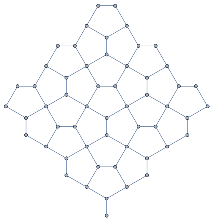
feg = IGMeshCellAdjacencyGraph[mesh, 1, 2,
VertexCoordinates -> Automatic]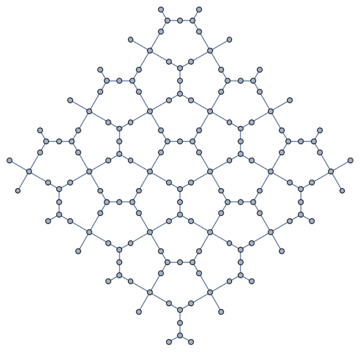
IGHomeomorphicQ[feg, ffg]False
feg = VertexDelete[feg, IGTreelikeComponents[feg]]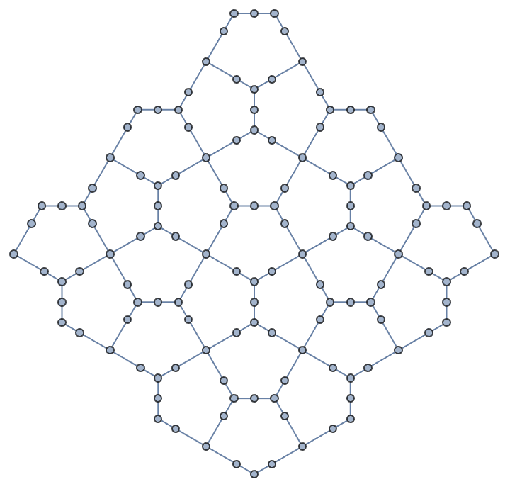
ffg = VertexDelete[ffg, IGTreelikeComponents[ffg]]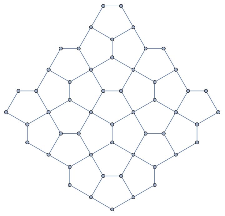
IGHomeomorphicQ[feg, ffg]True
?IGSelfComplementaryQ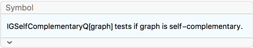
A graph is called self-complementary if it is isomorphic with its complement.
The 4-vertex path graph is self-complementary.
IGSelfComplementaryQ[PathGraph@Range[4]]True
Find all 3-vertex self-complementary directed graphs.
Select[IGData[{"AllDirectedGraphs", 3}], IGSelfComplementaryQ]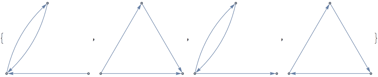
?IGColoredSimpleGraph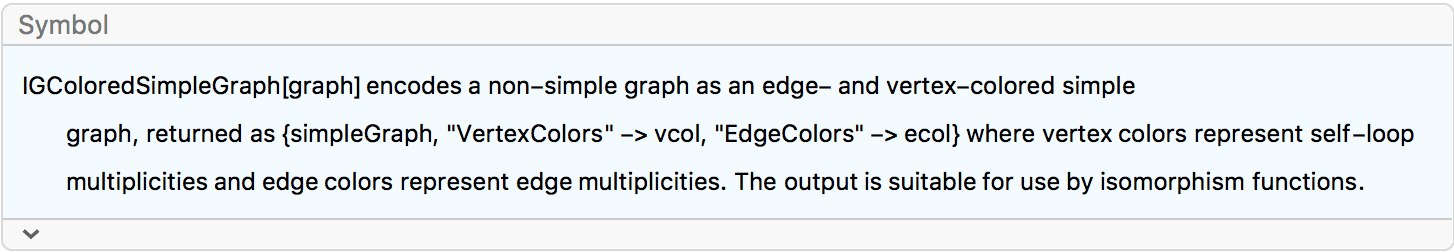
IGColoredSimpleGraph is a helper function that encodes a
non-simple graph (i.e a graph with self-loops or multi-edges) into an
edge- and vertex-colored simple graph. The coloured simple graph can be
used directly as an input to coloured isomorphism checking functions
such as IGVF2IsomorphicQ.
The vertex colours are computed as the multiplicity of self-loops at each vertex. The edge colours are computed as the multiplicities or non-loop edges.
The following graphs are not simple and cannot be used with
IGVF2IsomorphicQ directly.
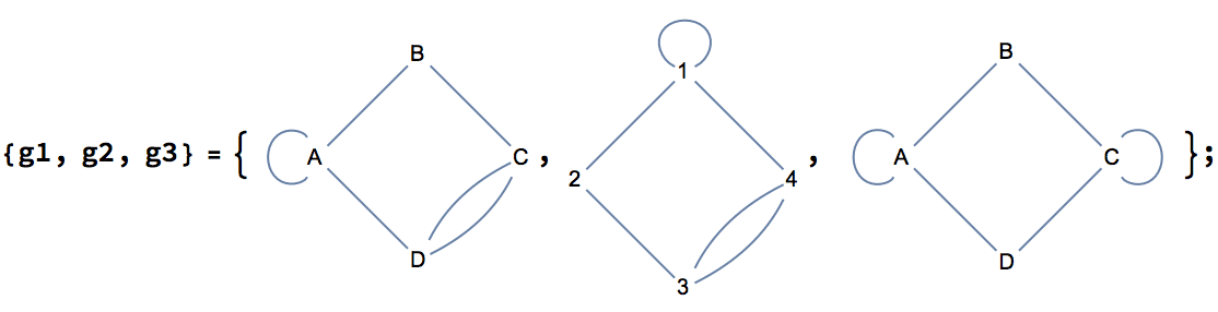
IGVF2IsomorphicQ[g1, g2]![]()
$Failed
IGColoredSimpleGraph can encode them as coloured graphs.
Its output can be supplied directly to
IGVF2IsomorphicQ.
IGColoredSimpleGraph[g1]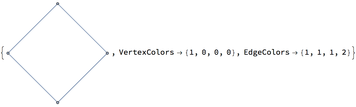
Now can can determine that g1 is isomorphic to
g2, but not to g3.
IGVF2IsomorphicQ[IGColoredSimpleGraph[g1], IGColoredSimpleGraph[g2]]True
IGVF2IsomorphicQ[IGColoredSimpleGraph[g1], IGColoredSimpleGraph[g3]]False
When searching for subgraphs in multigraphs with this method, be aware that a match occurs only if the edge multiplicities are the same. This sort of matching is useful e.g. in substructure search chemistry, where a double bond must only match another double bond, but not a single one.
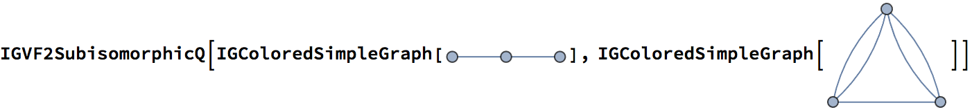
False
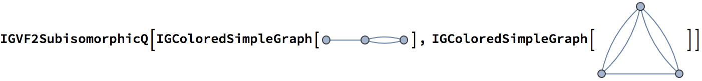
True
Use IGSubisomorphicQ to match any subgraph.
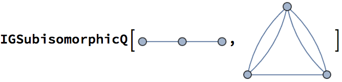
True
?IGMaximumFlowValue
IGMaximumFlowValue is equivalent to
IGMinimumCutValue except that it uses the
EdgeCapacity property instead of
EdgeWeight.
Edge capacities are taken from the EdgeCapacity
property.
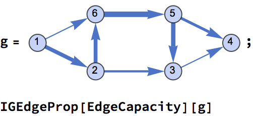
{3.5, 2, 1, 2.5, 5, 1, 3.5, 4}
IGMaximumFlowValue[g, 1, 4]3.5
?IGMaximumFlowMatrix
Element \(F_{ij}\) of the flow matrix is the flow through the edge connecting the \(i\)th node to the \(j\)th one. In an undirected graph, \(F_{ij}=-F_{ij}\).
Edge capacities are taken from the EdgeCapacity
property.
Let us take a directed graph with edge capacities set …
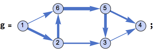
IGEdgeProp[EdgeCapacity][g]{3.5, 2, 1, 2.5, 5, 1, 3.5, 4}
… and compute the maximum flow between two of its vertices.
flowMat = IGMaximumFlowMatrix[g, 1, 4]![]()
The result is returned as a sparse matrix containing the flows through each edge.
MatrixForm[flowMat]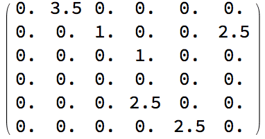
If the input is an undirected graph, the flow matrix contains entries of opposing sign for the two directions along each edge.
IGMaximumFlowMatrix[UndirectedGraph[g], 1, 4] // MatrixForm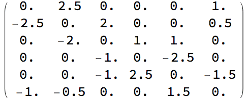
?IGMinimumCut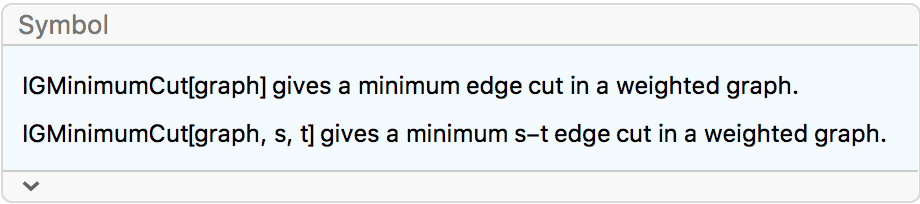
IGMinimumCut finds a single minimum edge cut in a
weighted graph. To find all minimum cuts between two given vertices, use
IGFindMinimumCuts.
?IGMinimumCutValue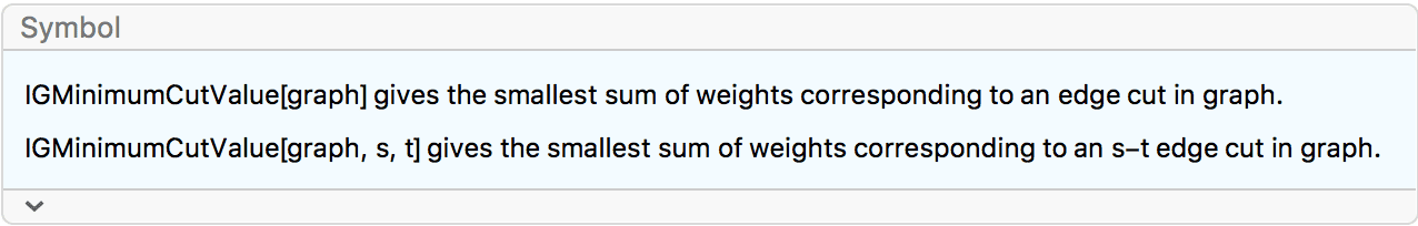
Unlike IGEdgeConnectivity,
IGMinimumCutValue takes weights into account.
IGMinimumCutValue[
Graph[{1 <-> 2, 2 <-> 3},
EdgeWeight -> {3.5, 5.6}]]3.5
The minimum cut value of the null graph and singleton graph are
returned as 0 and ∞, respectively.
IGMinimumCutValue /@ {IGEmptyGraph[0], IGEmptyGraph[1]}{0., ∞}
?IGGomoryHuTree
The Gomory–Hu tree is a weighted tree that encodes the minimum cuts between all pairs of vertices of an undirected graph. The Gomory–Hu tree has the same vertices as the graph it characterizes. The minimum cut between an \(s\)-\(t\) pair of the graph has the same size as smallest edge weight on the path from \(s\) to \(t\) in the Gomory–Hu tree.
Weighted graphs are supported.
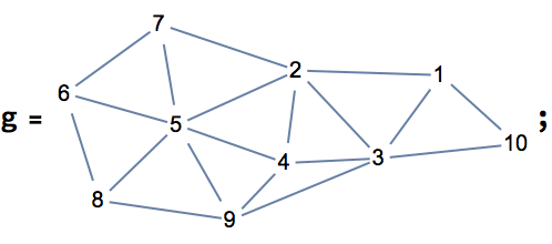
t = IGGomoryHuTree[g,
EdgeLabels -> "EdgeWeight", VertexShapeFunction -> "Name"
]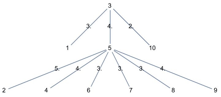
The path from 1 to 9 is
1 <-> 2 <-> 5 <-> 9 and has the weights
{3, 5, 4}. The smallest one, 3, is the minimum value of a
cut separating 1 from 9.
{IGMinimumCutValue[g, 1, 9], IGMinimumCutValue[t, 1, 9]}{3., 3.}
?IGCohesiveBlocks
The following examples are based on the ones in the R/igraph documentation.
This is the network from the Moody-White paper:
mw = Graph[{"1" <-> "2", "1" <-> "3",
"1" <-> "4", "1" <-> "5",
"1" <-> "6", "2" <-> "3",
"2" <-> "4", "2" <-> "5",
"2" <-> "7", "3" <-> "4",
"3" <-> "6", "3" <-> "7",
"4" <-> "5", "4" <-> "6",
"4" <-> "7", "5" <-> "6",
"5" <-> "7", "5" <-> "21",
"6" <-> "7", "7" <-> "8",
"7" <-> "11", "7" <-> "14",
"7" <-> "19", "8" <-> "9",
"8" <-> "11", "8" <-> "14",
"9" <-> "10", "10" <-> "12",
"10" <-> "13", "11" <-> "12",
"11" <-> "14", "12" <-> "16",
"13" <-> "16", "14" <-> "15",
"15" <-> "16", "17" <-> "18",
"17" <-> "19", "17" <-> "20",
"18" <-> "20", "18" <-> "21",
"19" <-> "20", "19" <-> "22",
"19" <-> "23", "20" <-> "21",
"21" <-> "22", "21" <-> "23",
"22" <-> "23"}, VertexLabels -> "Name"];{blocks, cohesion} = IGCohesiveBlocks[mw]{{{"1", "2", "3", "4", "5", "6", "7", "21", "8", "11", "14", "19", "9", "10", "12", "13", "16", "15", "17", "18", "20", "22", "23"}, {"1", "2", "3", "4", "5", "6", "7", "21", "19", "17", "18", "20", "22", "23"}, {"7", "8", "11", "14", "9", "10", "12", "13", "16", "15"}, {"1", "2", "3", "4", "5", "6", "7"}, {"7", "8", "11", "14"}}, {1, 2, 2, 5, 3}}
CommunityGraphPlot[mw, Rest@blocks,
CommunityRegionStyle ->
Table[Directive[Opacity[0.5], ColorData[96][i]], {i,
Length[blocks] - 1}]]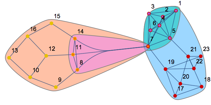
cohesion{1, 2, 2, 5, 3}
Science camp network:
sc = Graph[{"Pauline" <-> "Jennie",
"Pauline" <-> "Ann",
"Jennie" <-> "Ann",
"Jennie" <-> "Michael",
"Michael" <-> "Ann",
"Holly" <-> "Jennie",
"Jennie" <-> "Lee",
"Michael" <-> "Lee",
"Harry" <-> "Bert", "Harry" <-> "Don",
"Don" <-> "Bert", "Gery" <-> "Russ",
"Russ" <-> "Bert",
"Michael" <-> "John",
"Gery" <-> "John", "Russ" <-> "John",
"Holly" <-> "Pam", "Pam" <-> "Carol",
"Holly" <-> "Carol",
"Holly" <-> "Bill",
"Bill" <-> "Pauline",
"Bill" <-> "Michael",
"Bill" <-> "Lee", "Harry" <-> "Steve",
"Steve" <-> "Don",
"Steve" <-> "Bert",
"Gery" <-> "Steve",
"Russ" <-> "Steve",
"Pam" <-> "Brazey",
"Brazey" <-> "Carol", "Pam" <-> "Pat",
"Brazey" <-> "Pat",
"Carol" <-> "Pat", "Holly" <-> "Pat",
"Gery" <-> "Pat"}, VertexLabels -> "Name"];{blocks, cohesion} = IGCohesiveBlocks[sc]{{{"Pauline", "Jennie", "Ann", "Michael", "Holly", "Lee", "Harry", "Bert", "Don", "Gery", "Russ", "John", "Pam", "Carol", "Bill", "Steve", "Brazey", "Pat"}, {"Harry", "Bert", "Don", "Steve"}, {"Holly", "Pam", "Carol", "Brazey", "Pat"}, {"Pauline", "Jennie", "Ann", "Michael", "Lee", "Bill"}}, {2, 3, 3, 3}}
CommunityGraphPlot[sc, Rest@blocks,
CommunityRegionStyle -> ColorData[96], ImageSize -> Large]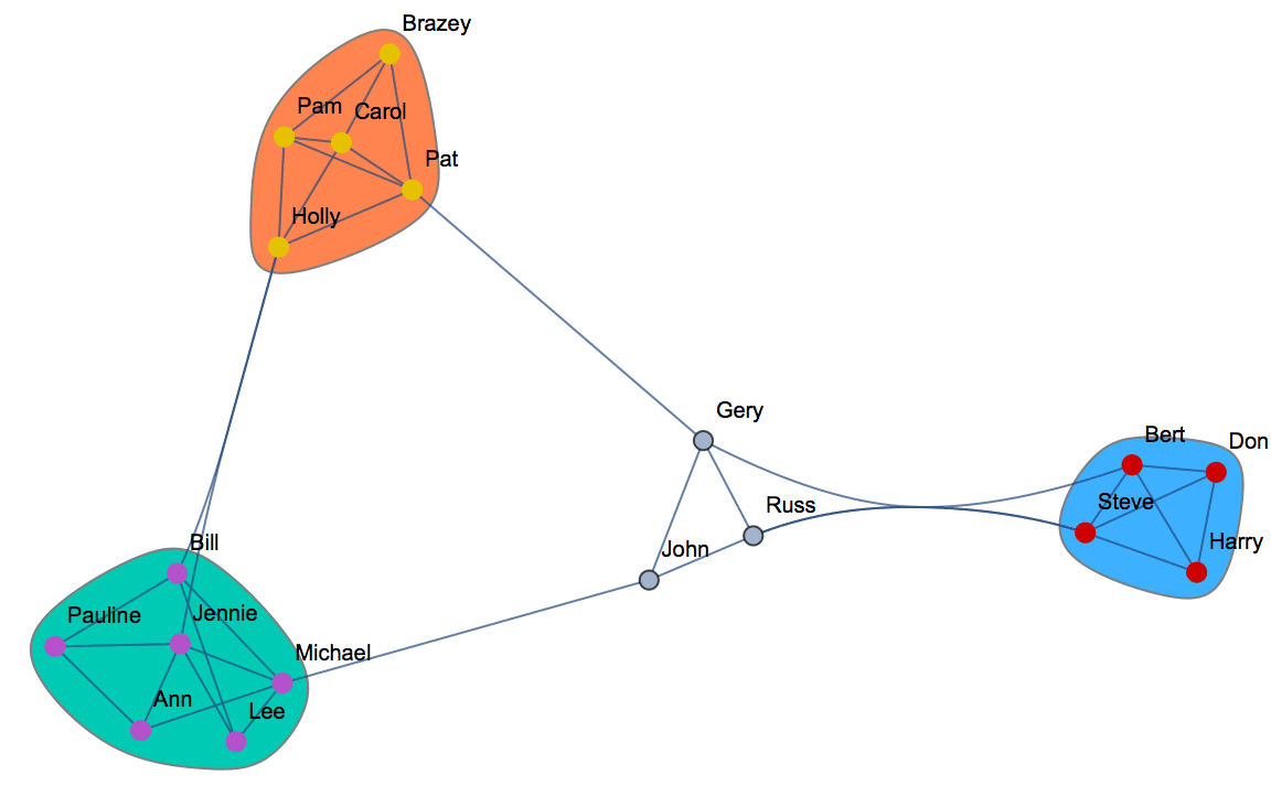
?IG*Clique*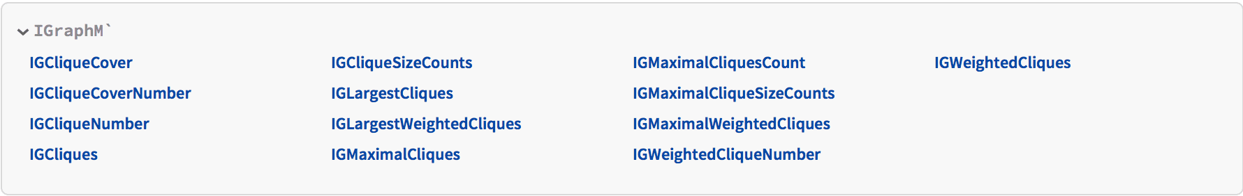
A clique is a fully connected subgraph. An independent vertex set is a subset of a graph’s vertices with no connections between them.
Mathematica’s FindClique function only finds
maximal cliques. IGraph/M provides functions for finding or counting all
cliques, i.e. complete subgraphs, of a graph.
g = ExampleData[{"NetworkGraph", "CoauthorshipsInNetworkScience"}];{VertexCount[g], EdgeCount[g]}{1589, 2742}
Simply counting cliques is much more memory efficient (and faster) than returning all of them.
IGCliqueSizeCounts[g]{1589, 2742, 3764, 7159, 17314, 39906, 78055, 126140, 167993, 184759, \ 167960, 125970, 77520, 38760, 15504, 4845, 1140, 190, 20, 1}
BarChart[%, ChartLabels -> Range@Length[%]]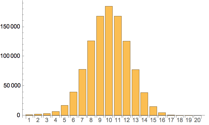
IGMaximalCliqueSizeCounts[g]{128, 221, 195, 108, 52, 19, 3, 8, 3, 3, 0, 0, 0, 0, 0, 0, 0, 0, 0, 1}
BarChart[%, ChartLabels -> Range@Length[%]]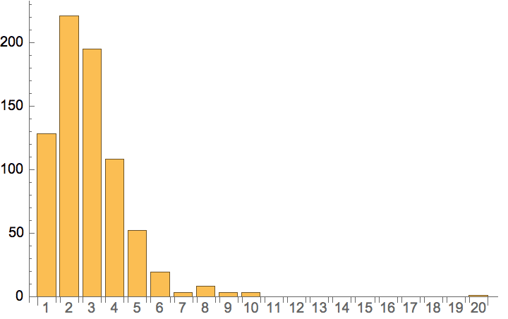
IGLargestCliques[g]{{"V. Narayan", "L. Giot", "J. Rothberg", "S. Fields", "M. Johnston", "M. Yang", "G. Vijayadamodar", "T. Kalbfleisch", "D. Conover", "B. Godwin", "Y. Li", "A. Qureshiemili", "P. Pochart", "M. Srinivasan", "D. Lockshon", "J. Knight", "R. Judson", "T. Mansfield", "G. Cagney", "P. Uetz"}}
The clique finder in IGraph/M ignores edge directions.
g = RandomGraph[{10, 60}, DirectedEdges -> True]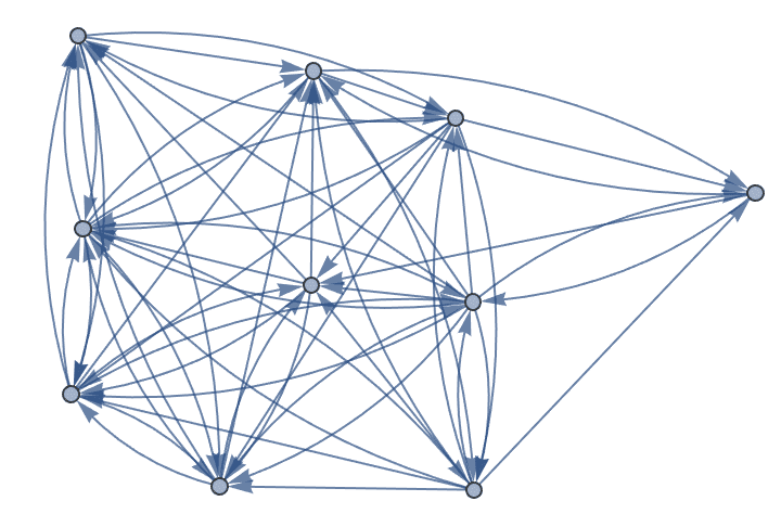
IGMaximalCliques[g]![]()
{{7, 2, 8, 6, 5, 3}, {2, 1, 10, 8, 6, 5, 4, 3}, {2, 1, 10, 8, 6, 5, 4, 9}}
To find cliques in directed graphs, convert them to undirected and keep mutual (bidirectional) edges only.
IGMaximalCliques@IGUndirectedGraph[g, "Mutual"]{{2, 7}, {2, 3, 4}, {6, 1, 10}, {7, 5}, {5, 4, 3}, {5, 4, 10, 1}, {8, 4, 3}, {8, 4, 9}, {9, 1, 10, 4}}
?IGCliqueCover
?IGCliqueCoverNumber
A clique cover of a graph is a partitioning of its vertices such that
each partition forms a clique. IGCliqueCover finds a
minimum clique cover, i.e. a partitioning into a smallest number of
cliques.
The clique cover number of a graph is the smallest number of cliques that can be used to cover its vertices.
Available Method option values are:
"Minimum" finds a minimum clique cover.
"Heuristic" is much faster, but the result is not
typically a minimum cover.
Compute a minimum clique cover of a random graph.
g = RandomGraph[{10, 20}]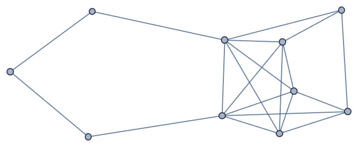
IGCliqueCover[g]{{1, 2, 6, 7}, {3, 5, 9}, {4, 10}, {8}}
Visualize the clique cover.
HighlightGraph[g, IGCliqueCover[g], VertexSize -> Large]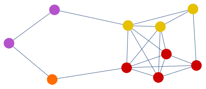
Find the clique cover number without returning a cover.
IGCliqueCoverNumber[g]4
The clique cover problem is equivalent to the colouring of the
complement graph. IGCliqueCover is effectively implemented
as
IGMembershipToPartitions[g]@IGMinimumVertexColoring@GraphComplement[g]{{1, 2, 6, 7}, {3, 5, 9}, {4, 10}, {8}}
For difficult problems, it may be useful to use
IGMinimumVertexColoring or IGVertexColoring
directly instead of IGCliqueCover, and tune their options
to achieve better performance. See the "ForcedColoring"
option of IGMinimumVertexColoring on how to do this.
g = ExampleData[{"NetworkGraph", "LesMiserables"}]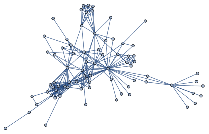
ExampleData[{"NetworkGraph", "LesMiserables"}, "LongDescription"]"Coappearance network of characters in the novel Les Miserables. \ EdgeWeight describes the number of coappearance."
The maximal cliques of the graph can approximate the scenes in which characters appear together.
cliques = IGMaximalCliques[g];We can construct a bipartite graph of connections between potential scenes and characters
IGLayoutBipartite[
Graph@Catenate[
Thread /@ Thread[Range@Length[cliques] <-> cliques]],
VertexSize -> 0.5, ImageSize -> 220
] // IGVertexMap[Placed[#, If[IntegerQ[#], Before, After]] &,
VertexLabels -> VertexList]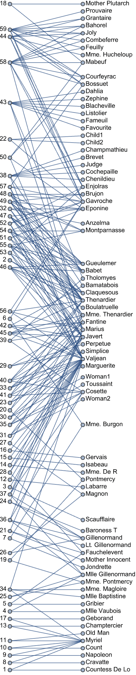
Note: The term “graphlet” is used for
multiple unrelated concepts in the literature. This section deals with
decomposing weighted graphs into cliques. If you are looking to count
induced subgraphs, see the IGMotifs
function.
?IGGraphlets
?IGGraphletBasis
?IGGraphletProject
g = IGShorthand["A,B,D,E,C, A-B-C-A, C-E-D-B, D-C, E-B",
EdgeWeight -> {2, 3, 2, 4, 4, 1, 4, 1},
EdgeLabels -> "EdgeWeight", VertexLabels -> None,
VertexShapeFunction -> "Name", PerformanceGoal -> "Quality",
GraphLayout -> "CircularEmbedding"
]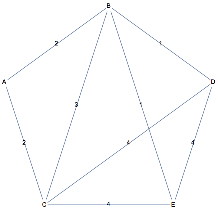
basis = IGGraphletBasis[g]<|{"A", "B", "C"} -> 2., {"B", "D", "E", "C"} -> 1., {"B", "C"} -> 3., {"D", "E", "C"} -> 4.|>
IGGraphletProject[g, Keys[basis]]<|{"A", "B", "C"} -> 0.925543, {"B", "D", "E", "C"} -> 0.861478, {"B", "C"} -> 2.90881*10^-253, {"D", "E", "C"} -> 1.13842| >
IGGraphlets[g]<|{"D", "E", "C"} -> 1.13842, {"A", "B", "C"} -> 0.925543, {"B", "D", "E", "C"} -> 0.861478, {"B", "C"} -> 2.90881*10^-253|>
The following functions are available:
?IGLayout*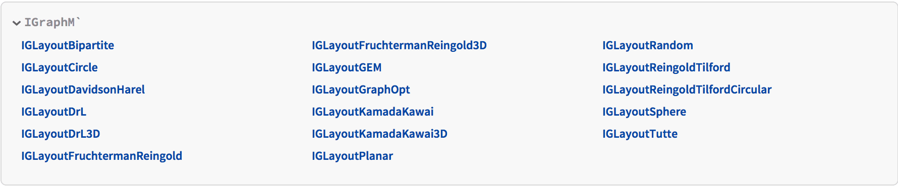
If you are looking for the Sugiyama layout from igraph, try the
built-in GraphLayout -> "LayeredDigraphEmbedding", or
LayeredGraphPlot. These are also based on the Sugiyama
algorithm.
Layout functions also take any standard Graph
option.
Many layout algorithms take the following options:
"MaxIterations" controls either the maximum
number of iterations performed by the algorithm or the exact
number of iterations, depending on the specific algorithm and settings.
The option name is the same for all functions to make it easier to
interchange them when visualizing dynamic graphs.
"Align" -> True aligns the output horizontally.
Examples:
{IGLayoutFruchtermanReingold[IGSquareLattice[{2, 4}](*,
"Align" -> True is the default *)],
IGLayoutFruchtermanReingold[IGSquareLattice[{2, 4}],
"Align" -> False]}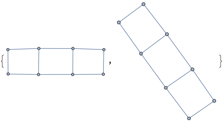
"Continue" -> True allows using existing vertex
coordinates as starting points for algorithms that update vertex
positions incrementally. We can use this to visualize how the layout
algorithms work …
g = IGLayoutRandom@
RandomGraph[BarabasiAlbertGraphDistribution[100, 1]];
ListAnimate@
NestList[
IGLayoutGraphOpt[#, "Continue" -> True, "MaxIterations" -> 80,
"Align" -> False] &, g, 40]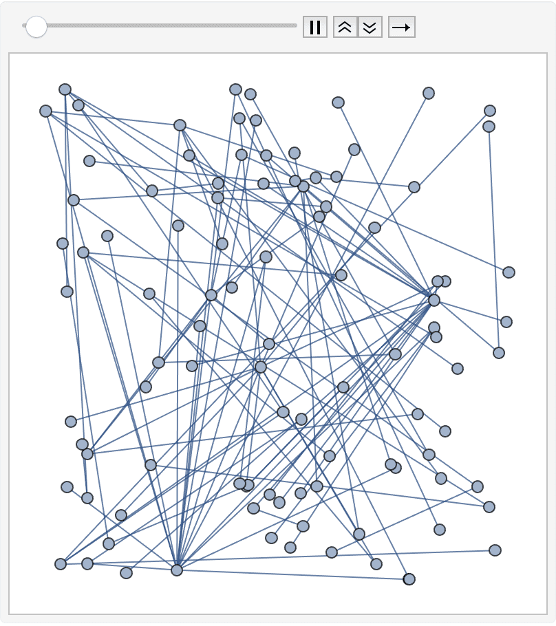
… or to visualize dynamic graph processes such as adding edges to the graph one by one:
g = IGLayoutKamadaKawai@
Graph[Range[25], {1 <-> 25},
VertexLabels -> "Name"];
ListAnimate@NestList[
IGLayoutKamadaKawai[
EdgeAdd[#, UndirectedEdge @@ RandomSample[VertexList[#], 2]],
"MaxIterations" -> 15, "Continue" -> True, "Align" -> False] &,
g,
30
]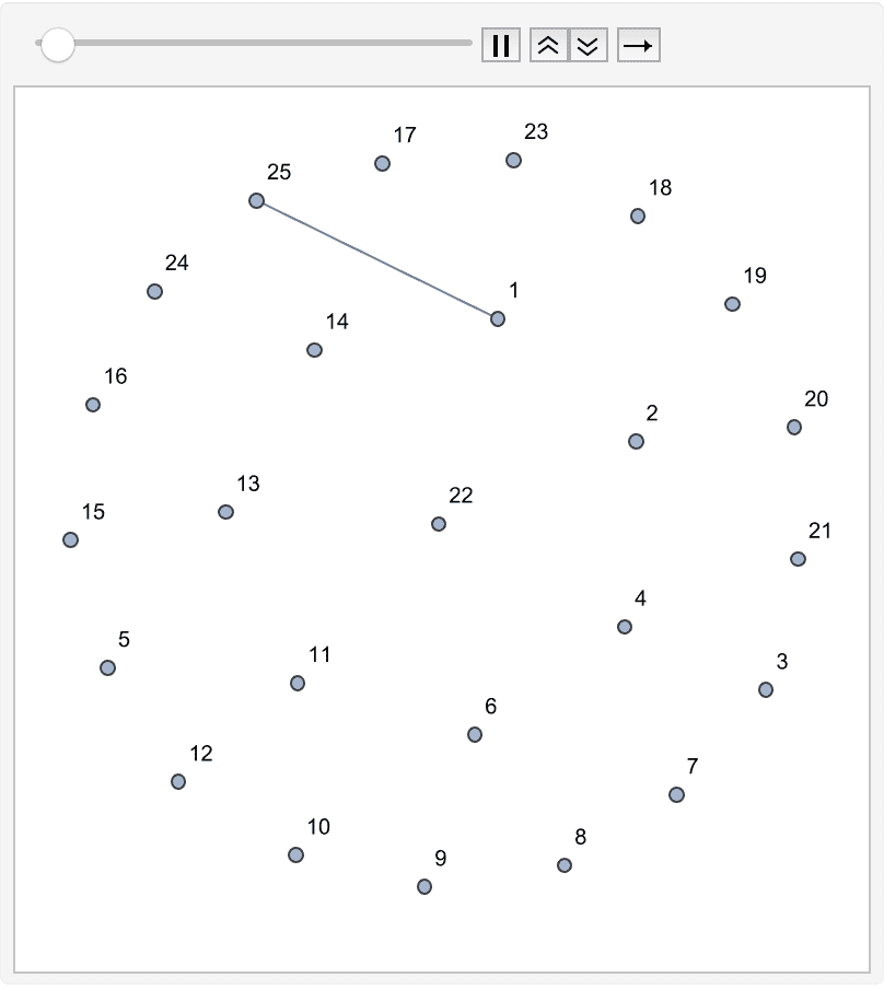
Visualize a planar graph without edge crossings using the
Davidson–Harel simulated annealing method, and taking starting
coordinates from GraphLayout -> "PlanarEmbedding".
g = Graph@GraphData[{"Fullerene", {60, 1}}, "EdgeList"]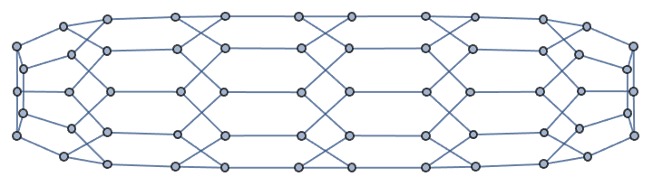
This layout avoids crossings, but it is not pleasing:
Graph[g, GraphLayout -> "PlanarEmbedding"]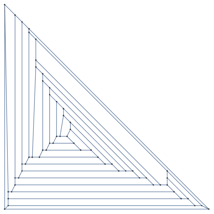
We can post process it while avoiding the introduction of any edge crossings:
IGLayoutDavidsonHarel[
IGVertexMap[# &,
VertexCoordinates -> (Rescale@
GraphEmbedding[#, "PlanarEmbedding"] &), g],
"Continue" -> True, "EdgeCrossingWeight" -> 1000
]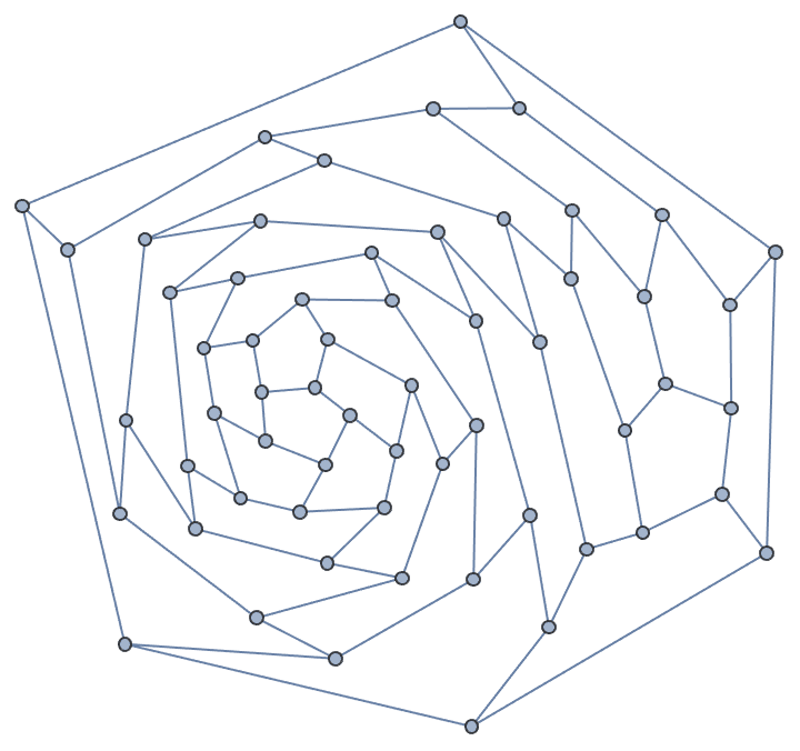
Several of the graph layout algorithms in igraph can take edge weights into accounts. How the weights are used during layout differs between them.
IGLayoutFruchtermanReingold multiplies the
attraction between vertices by the weights. Thus higher weights result
in shorter edges.
IGLayoutKamadaKawai produces longer edges for higher
weights
Graph layout functions which have a "Constraints" option
allow fixing the position of some vertices, or constraining them into a
box. This is an experimental feature that may change in the future.
The value of the "Constraints" option must be an
association from vertex names to vertex coordinates, or to bounding
boxes.
Fix the positions of three vertices and highlight them in red:
IGLayoutFruchtermanReingold[
IGShorthand["1:2:3:4 - 1:2:3:4:5, 5-6-7, 7:8:9 - 7:8:9"],
"Constraints" -> <|4 -> {-1, 0}, 7 -> {1, 0}, 6 -> {0, 1}|>,
VertexStyle -> {4 -> Red, 7 -> Red, 6 -> Red},
Frame -> True, FrameTicks -> True, GridLines -> Automatic
]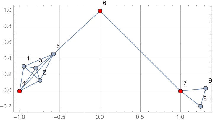
IGLayoutReingoldTilford[] and
IGLayoutReingoldTilfordCircular[] are designed for laying
out trees or forests. The following options are available:
"RootVertices" allows specifying the root node(s).
It must be a list, even if there is a single root node. Multiple root
nodes are meant to be used with forests. The roots should be selected so
that all vertices of the graph are reachable from them.
"RootVertices" -> Automatic chooses roots automatically,
preferring low eccentricity vertices in small graphs (fewer than 500
vertices) and high degree vertices in large graphs.
DirectedEdges -> False ignores edge directions.
By default, directed graphs are laid out so that edges are pointing away
from the root.
"Rotation" controls the orientation of the layout.
It must be given in radians.
The following options are unique to
IGLayoutReingoldTilford[]:
"LeafDistance" sets the spacing between tree leaves.
The default is 1.
"LayerHeight" sets the spacing between layers of the
drawing. The default is 1.
The same tree laid out in directed and undirected modes:
t = IGTreeGame[12, DirectedEdges -> True];
{IGLayoutReingoldTilford[t],
IGLayoutReingoldTilford[t, DirectedEdges -> False]}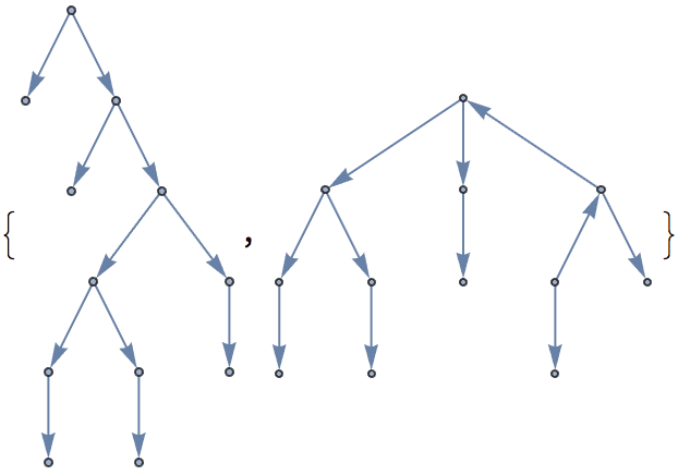
Lay out the tree radially, with successive layers places on circular shells:
IGLayoutReingoldTilfordCircular[t,
GraphStyle -> "Minimal",
Prolog -> {Thin, Gray,
Table[Circle[{0, 0}, r], {r,
IGDiameter[t, "ByComponents" -> True]}]}]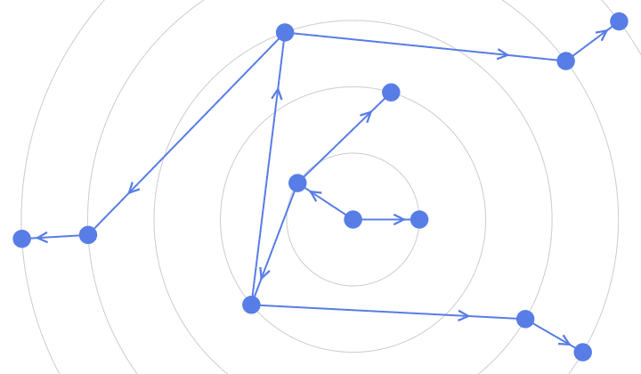
Use a left-to-right layout, with tightly spaced leaves:
IGLayoutReingoldTilford[t, "Rotation" -> Pi/2, "LeafDistance" -> 1/3]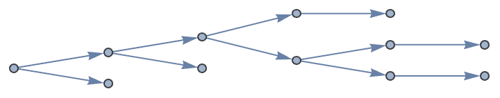
In an undirected tree, any vertex may be chosen as the root:
t = IGTreeGame[6];
Table[
IGLayoutReingoldTilford[t, "RootVertices" -> {r},
GraphStyle -> "DiagramGold"],
{r, VertexList[t]}
]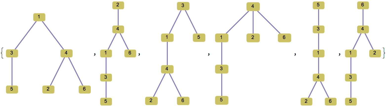
?IGLayoutBipartite
IGLayoutBipartite draws a bipartite graph, attempting to
minimize the number of edge crossing using the Sugiyama algorithm.
The available options are:
"Orientation" can be Horizontal or
Vertical
"PartitionGap" controls the size of the gap between
the two partitions
"VertexGap" controls the minimum size of the gap
between vertices in a partition
MaxIterations controls the maximum number of
iterations performed during edge crossing minimization.
"BipartitePartitions" can be used to explicitly
specify the partitioning of the graph.
IGLayoutBipartite[IGBipartiteGameGNP[10, 10, 0.2],
VertexLabels -> "Name"]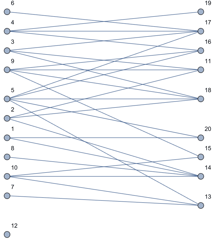
By default, a partitioning is computed automatically.
g = Graph[{1 <-> 2, 3 <-> 4},
VertexLabels -> "Name"];
IGLayoutBipartite[g]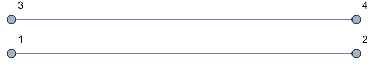
The partitioning can also be specified explicitly.
IGLayoutBipartite[g, "BipartitePartitions" -> {{2, 3}, {4, 1}}]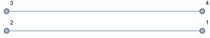
Draw a bipartite layout with curved edges.
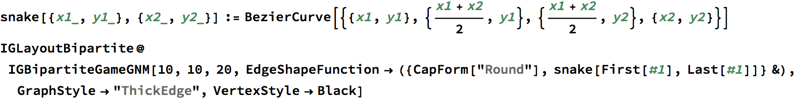
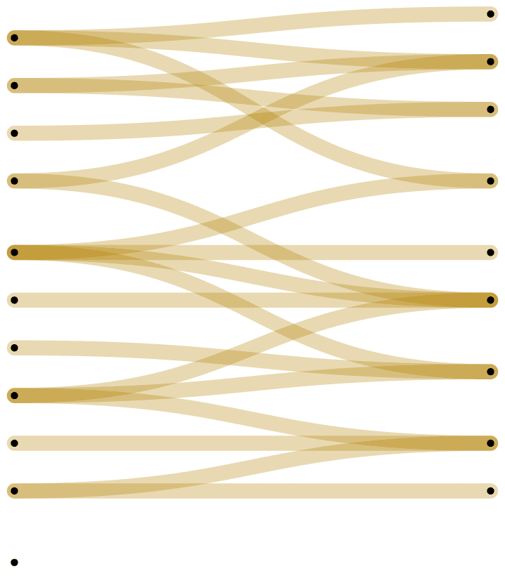
IGLayoutDrL is designed specifically for visualizing
large graphs with high clustering. The following image is created using
DrL and shows a 36000 node network of collaborations
between condensed matter scientists.
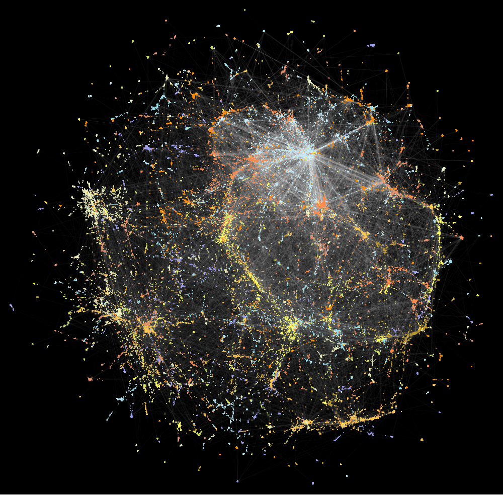
The image was generated using the following code:
lg = ExampleData[{"NetworkGraph",
"CondensedMatterCollaborations2005"}];
lg = IndexGraph@Subgraph[lg, First@ConnectedComponents[lg]];
c = IGCommunitiesMultilevel[lg]
pts = GraphEmbedding@IGLayoutDrL[lg]; (* this takes a while *)
figure = Graphics[
GraphicsComplex[pts,
{
{White, AbsoluteThickness[0.3], Opacity[0.05],
Line[List @@@ EdgeList[lg]]},
{AbsolutePointSize[2], Opacity[0.7],
MapIndexed[
{ColorData[45]@First[#2], Point[#1]} &,
c["Communities"]
]}
}
],
Background -> Black
]shift-enter evaluation is disabled in the cell above to avoid running it accidentally. Running the code takes about 2-3 minutes on a modern computer. Copy the code to a new cell to try it.
Create galleries of the various graph layouts available in IGraph/M.
Visualise a tree graph with all layouts.
g = IGBarabasiAlbertGame[32, 1, DirectedEdges -> False];
layouts =
Graph[#[g], PlotLabel -> #, LabelStyle -> 7] & /@ {IGLayoutCircle,
IGLayoutSphere, IGLayoutDavidsonHarel, IGLayoutDrL, IGLayoutDrL3D,
IGLayoutFruchtermanReingold, IGLayoutFruchtermanReingold3D,
IGLayoutGEM, IGLayoutGraphOpt, IGLayoutKamadaKawai,
IGLayoutKamadaKawai3D, IGLayoutRandom, IGLayoutReingoldTilford,
IGLayoutReingoldTilfordCircular, IGLayoutBipartite,
IGLayoutPlanar};
Multicolumn[layouts]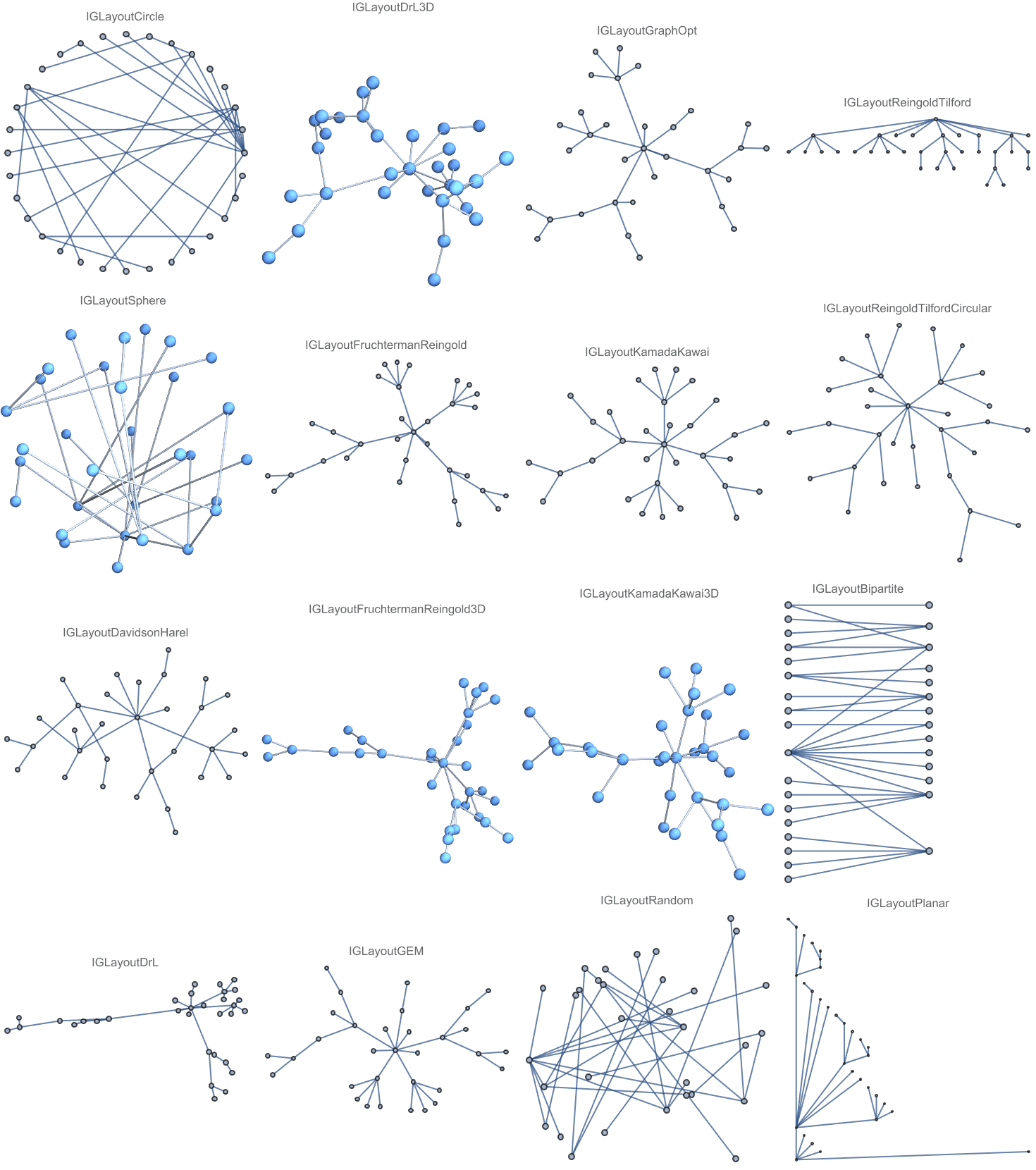
Visualise a polyhedral graph with all layouts.
g = GraphData["DodecahedralGraph"];
layouts =
Graph[#[g], PlotLabel -> #, LabelStyle -> 7] & /@ {IGLayoutCircle,
IGLayoutSphere, IGLayoutDavidsonHarel, IGLayoutDrL, IGLayoutDrL3D,
IGLayoutFruchtermanReingold, IGLayoutFruchtermanReingold3D,
IGLayoutGEM, IGLayoutGraphOpt, IGLayoutKamadaKawai,
IGLayoutKamadaKawai3D, IGLayoutRandom, IGLayoutPlanar,
IGLayoutTutte};
Multicolumn[layouts]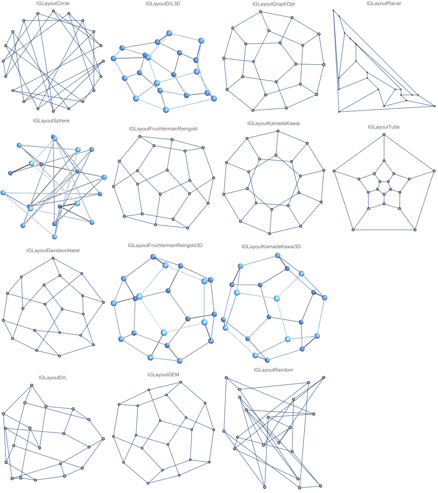
The following functions are available:
?IGCommunities*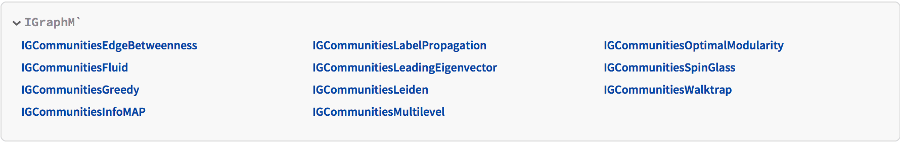
Modularity is defined for a given partitioning of a graph’s vertices into communities. For undirected graphs, it is defined as
\[Q=\frac{1}{2m}\sum _{i,j} \left(A_{ij}-\frac{k_ik_j}{2m}\right)\delta _{c_ic_j},\]
where \(m\) is the number of edges, \(A\) is the adjacency matrix, \(k_i\) is the degree of node \(i\), and \(c_i\) is the community that node \(i\) belongs to. \(\delta _{ij}\) is the Kronecker \(\delta\) symbol. For weighted graphs, \(A\) is the weighted adjacency matrix, \(k_i\) are the sum of weights of edges incident on node \(i\), and \(m\) is the sum of all weights.
Modularity characterizes the tendency of vertices to connect more
within their own group than with other groups, relative to a null model
that considers vertex degrees to be fixed. For a given partitioning, it
can be computed using IGModularity. Most community
detection methods aim find a partitioning of the graph which results in
high modularity.
Community detection functions return IGClusterData
objects.
g = ExampleData[{"NetworkGraph", "FamilyGathering"}]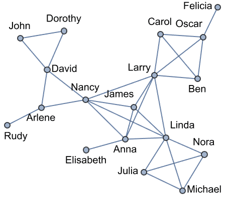
cl = IGCommunitiesGreedy[g]![]()
The data available in the object can be queried using
IGClusterData[…]["Properties"]. See the Examples section
below for more information. In Mathematica 12.0 and later, Information
can be used to get a quick human-readable summary.
cl["Properties"]{"Algorithm", "Communities", "ElementCount", "Elements", \ "HierarchicalClusters", "Merges", "Modularity", "Properties", "Tree"}
cl["Communities"]{{"Elisabeth", "James", "Anna", "Nancy"}, {"John", "Dorothy", "David", "Arlene", "Rudy"}, {"Linda", "Michael", "Nora", "Julia"}, {"Larry", "Carol", "Ben", "Oscar", "Felicia"}}
CommunityGraphPlot[g, cl["Communities"], ImageSize -> Medium]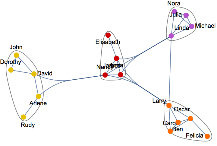
IGModularity[g, cl]0.454735
?IGClusterData
IGClusterData represents a partitioning of a graph into
communities. This object cannot be created directly. It is returned by
community detection functions. See the Examples section below for more
information.
cl = IGCommunitiesLabelPropagation@
ExampleData[{"NetworkGraph", "FamilyGathering"}]![]()
Query the available properties.
cl["Properties"]{"Algorithm", "Communities", "ElementCount", "Elements", \ "Modularity", "Properties"}
Retrieve the communities.
cl["Communities"]{{"Elisabeth", "James", "Anna", "Linda", "Larry", "Carol", "Nancy", "David", "Ben", "Oscar", "Felicia", "Arlene", "Rudy"}, {"John", "Dorothy"}, {"Michael", "Nora", "Julia"}}
When the "Modularity" property is available,
Max[cl["Modularity"]] gives the modularity of the current
partitioning.
Max[cl["Modularity"]]0.188866
?IGModularity
IGModularity computes the generalized modularity in
undirected or directed graphs, taking weights into account. For
undirected graphs, it is defined as
\[Q=\frac{1}{2m}\sum _{i,j} \left(A_{ij}-\gamma \frac{k_ik_j}{2m}\right)\delta _{c_ic_j},\]
where \(m\) is the number of edges, \(A\) is the adjacency matrix, \(k_i\) is the degree of node \(i\), and \(c_i\) is the community that node \(i\) belongs to. \(\delta _{ij}\) is the Kronecker \(\delta\) symbol. For weighted graphs, \(A\) is the weighted adjacency matrix, \(k_i\) are the sum of weights of edges incident on node \(i\), and \(m\) is the sum of all weights. In the undirected case, \(A_{ii}\) is assumed to contain twice the number of self-loops on vertex \(i\), or twice their total weight in the weighted case. \(\gamma\) is a resolution parameter, with \(\gamma =1\) yielding the standard modularity.
The directed generalization is
\[Q=\frac{1}{m}\sum _{i,j} \left(A_{ij}-\gamma \frac{k_i^{\text{out}}k_j^{\text{in}}}{m}\right)\delta _{c_ic_j}.\]
For simple graphs, IGModularity[graph, communities] is
equivalent to
GraphAssortativity[graph, communities, "Normalized" -> False].
However, in contrast to GraphAssortativity,
IGModularity does take self-loops and multi-edges into
account.
Available options are:
"Resolution" -> γ sets the resolution parameter.
The default is 1.
DirectedEdges -> True takes into account edge
directions in directed graphs. By default, they are ignored.
Compute the modularity of a stochastic block model graph having three partitions, each with 20 vertices.
![]()
IGModularity[g, Partition[VertexList[g], 20]]0.456154
Setting the resolution parameter to zero computes the fraction of intra-community edges.
IGModularity[g, Partition[VertexList[g], 20], "Resolution" -> 0]0.8125
?IGModularityMatrix
IGModularityMatrix computes the generalized modularity
matrix of a graph, defined as
\[B_{ij}=A_{ij}-\gamma \frac{k_ik_j}{2m}\]
for undirected graphs and as
\[B_{ij}=A_{ij}-\gamma \frac{k_i^{\text{out}}k_j^{\text{in}}}{m}\]
for directed ones. Here, \(A\)
represents the adjacency matrix, \(k_i\) is the degree of vertex \(i\), \(m\)
is the sum of edge weights and \(\gamma\) is the resolution parameter. Just
as with IGModularity, in undirected graphs \(A_{ii}\) is assumed to contain twice the
number of self-loops. This way, the result for an undirected graph is
the same as for the corresponding directed one where all undirected
edges are replaced by a pair of reciprocal directed ones.
Available options are:
"Resolution" -> γ sets the resolution parameter.
The default is 1.
DirectedEdges -> True takes into account edge
directions in directed graphs. By default, they are ignored.
The modularity matrix is used in spectral clustering algorithms, such
as the one implemented by IGCommunitiesLeadingEigenvector.
Communities can be separated based on spatial clustering of the points
formed by the first few eigenvectors of the modularity matrix.
g = IGStochasticBlockModelGame[
0.05 + 0.5 IdentityMatrix[3], {10, 10, 10}]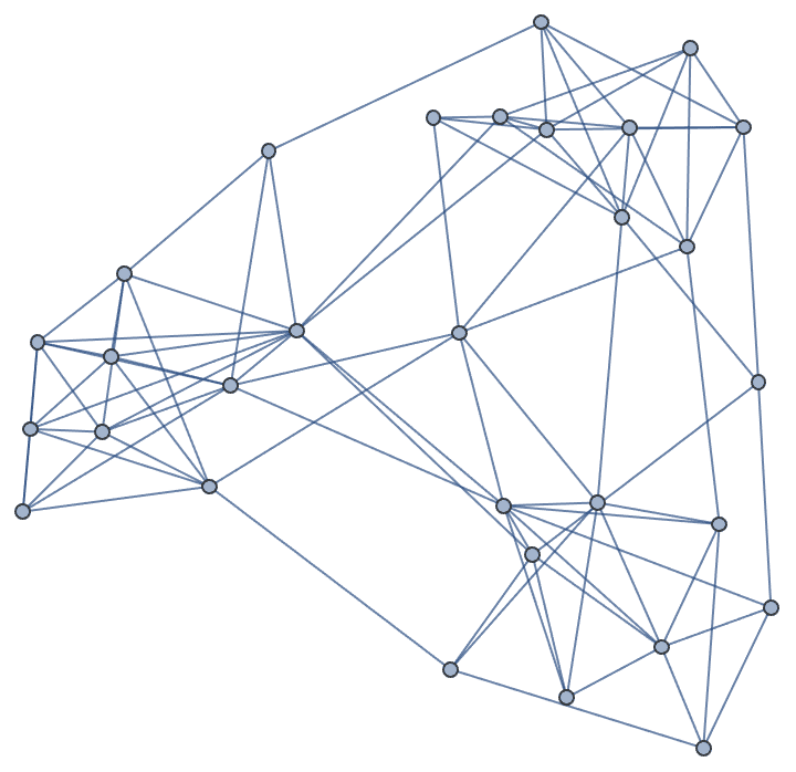
ListPlot[
FindClusters@Transpose@Eigenvectors[IGModularityMatrix[g], 2],
PlotStyle -> PointSize[Large], AspectRatio -> Automatic]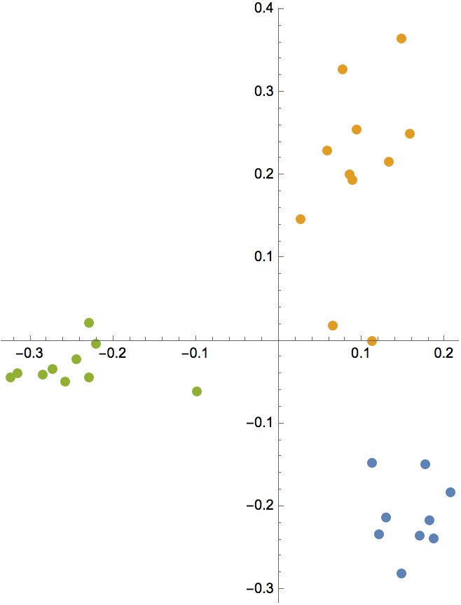
?IGCompareCommunities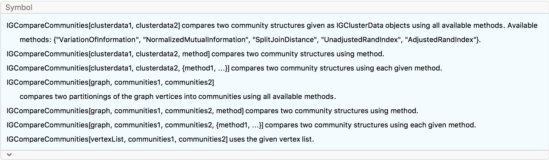
Some of these measures are defined based on the entropy of a discrete random variable associated with a given clustering \(C\) of vertices. Let \(p_i\) be the probability that a randomly picked vertex would be part of cluster \(i\). Then the entropy of the clustering is
\[H(C)=-\sum _ip_i\ln p_i.\]
Similarly, we can define the joint entropy of two clusterings \(C_1\) and \(C_2\) based on the probability \(p_{ij}\) that a random vertex is part of cluster \(i\) in the first clustering and cluster \(j\) in the second one:
\[H\left(C_1,C_2\right)=-\sum _{i,j}p_{ij}\ln p_{ij}.\]
The mutual information of \(C_1\) and \(C_2\) is then \(\text{MI}\left(C_1,C_2\right)=H\left(C_1\right)+H\left(C_2\right)-H\left(C_1,C_2\right)\text{$>$=}0\). A large mutual information indicates a high overlap between the two clusterings. The normalized mutual information, as computed by igraph, is
\[\text{NMI}\left(C_1,C_2\right)=\frac{2\text{MI}\left(C_1,C_2\right)}{H\left(C_1\right)+H\left(C_2\right)}.\]
It takes its value from the interval \((0,1]\), with 1 achieved when the two clusterings coincide.
The variation of information is defined as \(\text{VI}\left(C_1,C_2\right)=\left[H\left(C_1\right)-\text{MI}\left(C_1,C_2\right)\right]+\left[H\left(C_2\right)-\text{MI}\left(C_1,C_2\right)\right]=2H\left(C_1,C_2\right)-H\left(C_1\right)-H\left(C_2\right)\). Lower values of the variation of information indicate a smaller difference between the two clusterings, with \(\text{VI}=0\) achieved precisely when they coincide.
The Rand index is defined based on counting pairs of vertices that are within the same or different clusters in the two clusterings. Let \(a_1\) and \(a_2\) denote the number of pairs that are grouped together in \(C_1\) and \(C_2\), respectively. Then the Rand index is
\[\text{RI}\left(C_1,C_2\right)=\frac{a_1+a_2}{\left( \begin{array}{c} n \\ 2 \\ \end{array} \right)},\]
where \(\left( \begin{array}{c} n \\ 2 \\ \end{array} \right)\) is the total number of pairs of \(n\) vertices. The value of the Rand index varies between 0 and 1. The adjusted Rand index, \(\text{ARI}\), corrects the value based on the Rand index expected after after a random rearrangement of the vertices, denoted \(\text{ERI}\):
\[\text{ARI} = \frac{\text{RI}-\text{ERI}}{1-\text{ERI}}.\]
g = ExampleData[{"NetworkGraph", "FamilyGathering"}];{cl1, cl2} = {IGCommunitiesGreedy[g], IGCommunitiesEdgeBetweenness[g]}![]()
IGCompareCommunities[cl1, cl2]<|"VariationOfInformation" -> 0.278001, "NormalizedMutualInformation" -> 0.899283, "SplitJoinDistance" -> 2, "UnadjustedRandIndex" -> 0.947712, "AdjustedRandIndex" -> 0.841942|>
?IGCommunitiesEdgeBetweenness
IGCommunitiesEdgeBetweenness[] implements the
Girvan–Newman algorithm.
Weighted graphs are supported. Weights are treated as “distances”, i.e. a large weight represents a weak connection.
Available option values:
"ClusterCount", the number of communities to return.
Default: Automatic.Special properties returned with the result:
"RemovedEdges" is the list of edges removed in each
step of the algorithm.
"Bridges" records the steps which resulted in
splitting the graph into more components.
?IGCommunitiesFluid
IGCommunitiesFluid[] implements the fluid communities
algorithm.
?IGCommunitiesGreedy
IGCommunitiesGreedy[] implements greedy optimization of
modularity.
Weighted graphs are supported.
?IGCommunitiesInfoMAP
IGCommunitiesInfoMAP[] implements the InfoMAP
algorithm.
It supports both edge weights and vertex weights.
The default number of trials is 10.
Special properties returned with the result:
"CodeLength" is the code length of the partition.M. Rosvall and C. T. Bergstrom, Maps of information flow reveal community structure in complex networks, PNAS 105, 1118 (2008)
M. Rosvall, D. Axelsson, and C. T. Bergstrom, The map equation, Eur. Phys. J. Special Topics 178, 13 (2009)
?IGCommunitiesLabelPropagation
Weighted graphs are supported.
?IGCommunitiesLeadingEigenvector
Weighted graphs are supported.
Available option values:
"ClusterCount", the number of communities to return.
May return fewer communities than requested. Default:
Automatic.?IGCommunitiesMultilevel
IGCommunitiesMultilevel[] implements the Louvain
community detection method.
Weighted graphs are supported.
?IGCommunitiesLeiden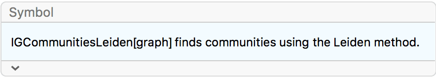
The Leiden algorithm is similar to the multilevel algorithm, often called the Louvain algorithm, but it is faster and yields higher quality solutions. It can optimize both modularity and the Constant Potts Model, which does not suffer from the resolution-limit (see preprint http://arxiv.org/abs/1104.3083).
The Leiden algorithm consists of three phases: (1) local moving of nodes, (2) refinement of the partition and (3) aggregation of the network based on the refined partition, using the non-refined partition to create an initial partition for the aggregate network. In the local move procedure in the Leiden algorithm, only nodes whose neighborhood has changed are visited. The refinement is done by restarting from a singleton partition within each cluster and gradually merging the subclusters. When aggregating, a single cluster may then be represented by several nodes (which are the subclusters identified in the refinement).
The Leiden algorithm provides several guarantees. The Leiden algorithm is typically iterated: the output of one iteration is used as the input for the next iteration. At each iteration all clusters are guaranteed to be connected and well-separated. After an iteration in which nothing has changed, all nodes and some parts are guaranteed to be locally optimally assigned. Finally, asymptotically, all subsets of all clusters are guaranteed to be locally optimally assigned.
The Leiden method maximizes a quality measure (a generalization of modularity) defined as
\[Q=\frac{1}{2m}\sum _{i,j}\left(A_{ij}-\gamma n_in_j\right)\delta _{c_ic_j}\]
where \(m\) is the sum of edge weights (number of edges if the graph is unweighted), \(A\) is the weighted adjacency matrix, \(n_i\) is the weight of vertex \(i\), and \(c_i\) is the community that vertex \(i\) belongs to. \(\delta _{ij}\) is the Kronecker \(\delta\) symbol.
\(\gamma\) is a resolution parameter
that can be set with the "Resolution" option.
The function chooses the vertex weights automatically, according to
the value of the VertexWeight option:
VertexWeight -> "NormalizedStrength" (default)
sets \(n_i=k_i/\sqrt{2m}\), where \(k_i\) is the strength (sum of incident edge
weights) of vertex \(i\). If \(\gamma =1\), then the quality measure
becomes equivalent to the modularity.
VertexWeight -> "Constant" sets \(n_i=1\). With this choice, it is
recommended to set the resolution parameter \(\gamma\) explicitly. A reasonable \(\gamma\) value for unweighted graphs is the
graph density.
VertexWeight -> "VertexWeight" takes vertex
weights from the VertexWeight graph property.
Other available options:
"Resolution" -> γ sets the resolution parameter
\(\gamma\). The default is \(\gamma =1\). With
VertexWeight -> "NormalizedStrength", a reasonable value
is 1. With VertexWeight -> "Constant", a reasonable
value is the graph density.
"Beta" -> β sets the randomness used in the
refinement step when merging clusters. The default is \(\beta =0.01\).
Special properties returned with the result :
"Quality" is the value of the quality measure \(Q\).Examples:
g = Graph[ExampleData[{"NetworkGraph", "LesMiserables"}],
GraphStyle -> "BasicBlack", VertexSize -> 2];With the default option values
VertexWeight -> "NormalizedStrength" and
"Resolution" -> 1, IGCommunitiesLeiden
effectively uses the modularity as the quality measure.
cl = IGCommunitiesLeiden[g]![]()
{cl["Quality"], IGModularity[g, cl]}{0.566688, 0.566688}
HighlightGraph[g, cl["Communities"]]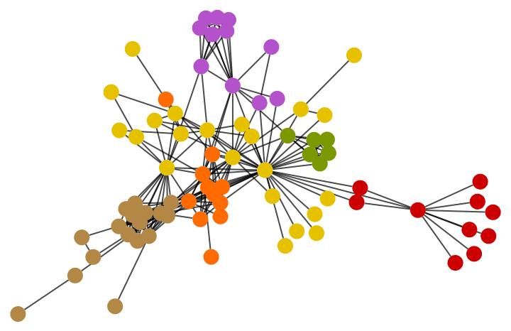
A higher "Resolution" value results in more
communities.
HighlightGraph[
g,
IGCommunitiesLeiden[g, "Resolution" -> 3]["Communities"]
]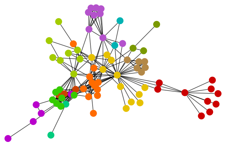
With VertexWeight -> "Constant", it is recommended to
set "Resolution" explicitly. A reasonable starting point is
GraphDensity[g].
HighlightGraph[
g,
IGCommunitiesLeiden[g, VertexWeight -> "Constant",
"Resolution" -> 0.1]["Communities"]
]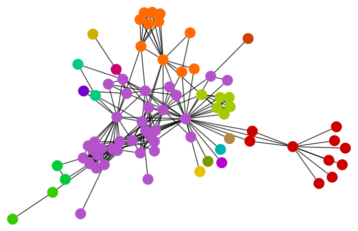
?IGCommunitiesOptimalModularity
Finds the clustering that maximizes modularity exactly. This algorithm is very slow.
Weighted graphs are supported.
?IGCommunitiesSpinGlass
Weighted graphs are supported.
Option values for Method are:
"Original" only supports positive edge weights, but
doesn’t check that the supplied weights are actually positive.
"Negative" supports negative weights as
well.
Automatic selects "Negative" if
negative weights are presents and "Original"
otherwise.
Option values for "UpdateRule" are:
"Simple", "Configuration"
Special properties returned with the result:
"FinalTemperature" is the final temperature at the end
of the algorithm.For Method -> "Original, see Joerg Reichardt and
Stefan Bornholdt: Statistical Mechanics of Community Detection, http://arxiv.org/abs/cond-mat/0603718
For Method -> "Negative", see V. A. Traag and
Jeroen Bruggeman: Community detection in networks with positive and
negative links, http://arxiv.org/abs/0811.2329
?IGCommunitiesWalktrap
IGCommunitiesWalktrap[] finds communities using short
random walks, exploiting the fact that random walks tend to stay within
the same cluster.
Weighted graphs are supported.
The default number of steps is 4.
Available option values:
"ClusterCount", the number of communities to return.
Default: Automatic.g = ExampleData[{"NetworkGraph", "LesMiserables"}]
IGEdgeWeightedQ[g]True
Community detection functions return IGClusterData
objects.
cl1 = IGCommunitiesEdgeBetweenness[g, "ClusterCount" -> 7]
cl2 = IGCommunitiesWalktrap[g]![]()
![]()
Various properties of these objects can be queried:
cl1["Communities"]{{"Myriel", "Napoleon", "Mlle Baptistine", "Mme. Magloire", "Countess De Lo", "Geborand", "Champtercier", "Cravatte", "Count", "Old Man"}, {"Labarre", "Valjean", "Marguerite", "Mme. De R", "Isabeau", "Gervais", "Bamatabois", "Perpetue", "Simplice", "Scaufflaire", "Woman1", "Judge", "Champmathieu", "Brevet", "Chenildieu", "Cochepaille"}, {"Tholomyes", "Listolier", "Fameuil", "Blacheville", "Favourite", "Dahlia", "Zephine", "Fantine"}, {"Mme. Thenardier", "Thenardier", "Cosette", "Javert", "Boulatruelle", "Eponine", "Anzelma", "Woman2", "Gueulemer", "Babet", "Claquesous", "Montparnasse", "Toussaint", "Brujon"}, {"Fauchelevent", "Mother Innocent", "Gribier"}, {"Pontmercy", "Gillenormand", "Magnon", "Mlle Gillenormand", "Mme. Pontmercy", "Mlle Vaubois", "Lt. Gillenormand", "Marius", "Baroness T"}, {"Jondrette", "Mme. Burgon", "Gavroche", "Mabeuf", "Enjolras", "Combeferre", "Prouvaire", "Feuilly", "Courfeyrac", "Bahorel", "Bossuet", "Joly", "Grantaire", "Mother Plutarch", "Child1", "Child2", "Mme. Hucheloup"}}
Visualize the detected communities in two different ways:
CommunityGraphPlot[g, cl1["Communities"]]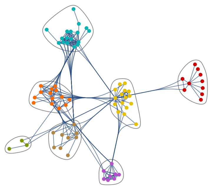
HighlightGraph[g, Subgraph[g, #] & /@ cl1["Communities"],
GraphHighlightStyle -> "DehighlightGray"]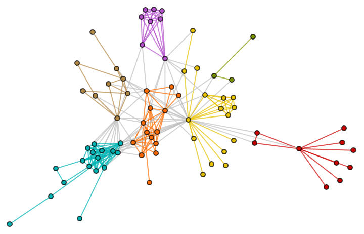
Plot the adjacency matrix, reordered to show the community structure.
IGAdjacencyMatrixPlot[g, Catenate@cl1["Communities"]]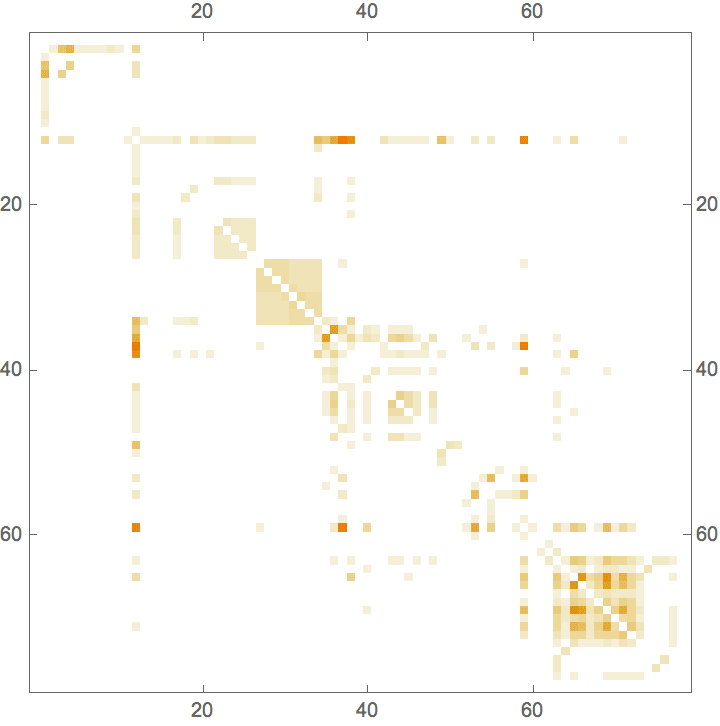
The available properties depend on which algorithm was used for community detection. The following are always present:
"Properties" returns all available
properties.
"Algorithm" returns the algorithm used for community
detection.
"Communities" returns the list of
communities.
"Elements" returns the vertices of the
graph.
"ElementCount" returns the vertex count of the
graph.
These are present for hierarchical clustering methods:
"HierarchicalClusters" returns the clustering in a
format compatible with the Hierarchical Clustering standard package.
Note: Isolated vertices may not be included.
"Merges" represents the hierarchical clustering as a
sequence of element merges. Elements are represented by their integer
indices, and higher indices are introduced for the subclusters formed by
the merges. This format is similar to the one used by MATLAB and many other tools.
Note: Isolated vertices may not be included.
"Tree" gives a binary tree representation of the
merges. Note: Isolated vertices may not be
included.
Additionally, the following, and other, algorithm-specific properties may be present:
"Modularity" is a list of modularities for each step of
the algorithm, or a single-element list containing the modularity
corresponding to the returned clustering. What constitutes a step
depends on the particular algorithm.The "RemovedEdges" property is specific to the
"EdgeBetweenness" method, and isn’t present for
"Walktrap".
cl1["Properties"]{"Algorithm", "Bridges", "Communities", "EdgeBetweenness", \ "ElementCount", "Elements", "HierarchicalClusters", "Merges", \ "Properties", "RemovedEdges", "Tree"}
Take[cl1["RemovedEdges"], 10]{"Valjean" <-> "Myriel", "Valjean" <-> "Mlle Baptistine", "Valjean" <-> "Mme. Magloire", "Gavroche" <-> "Valjean", "Gavroche" <-> "Javert", "Thenardier" <-> "Fantine", "Bamatabois" <-> "Javert", "Bossuet" <-> "Valjean", "Montparnasse" <-> "Valjean", "Gueulemer" <-> "Gavroche"}
cl2["Properties"]{"Algorithm", "Communities", "ElementCount", "Elements", \ "HierarchicalClusters", "Merges", "Modularity", "Properties", "Tree"}
Multiple properties may be retrieved at the same time.
cl2[{"Algorithm", "ElementCount"}]{"Walktrap", 77}
Compare the two clusterings:
IGCompareCommunities[cl1, cl2]<|"VariationOfInformation" -> 0.804544, "NormalizedMutualInformation" -> 0.786844, "SplitJoinDistance" -> 29, "UnadjustedRandIndex" -> 0.879699, "AdjustedRandIndex" -> 0.555464|>
Visualize the hierarchical clustering using the Hierarchical Clustering Package.
<< HierarchicalClustering`DendrogramPlot[cl1["HierarchicalClusters"],
LeafLabels -> (Rotate[#, Pi/2] &), ImageSize -> 750,
AspectRatio -> 1/2]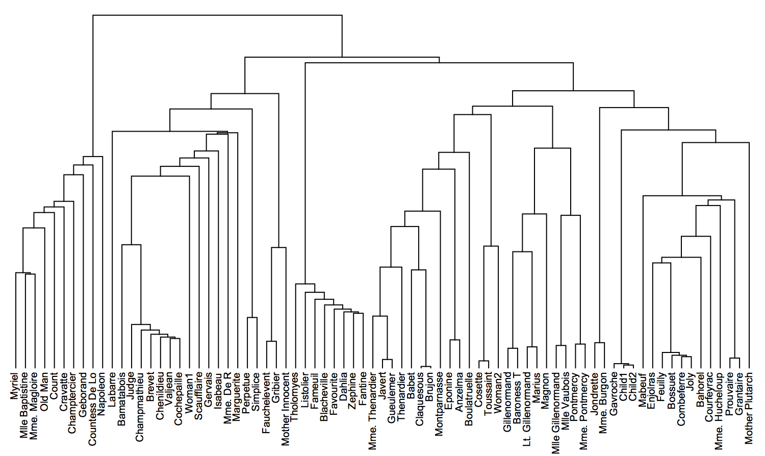
Hierarchical community structures can also be obtained as a vertex-weighted tree graph.
g = ExampleData[{"NetworkGraph", "ZacharyKarateClub"}];cl = IGCommunitiesGreedy[g];clusteringTree = cl["Tree"]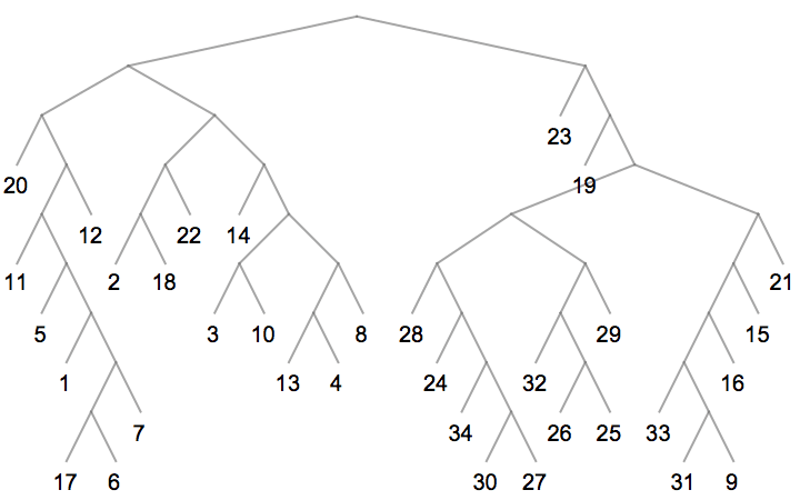
{GraphQ[clusteringTree], IGVertexWeightedQ[clusteringTree]}{True, True}
This tree can be supplied as input to Dendrogram.
Dendrogram[clusteringTree, Left]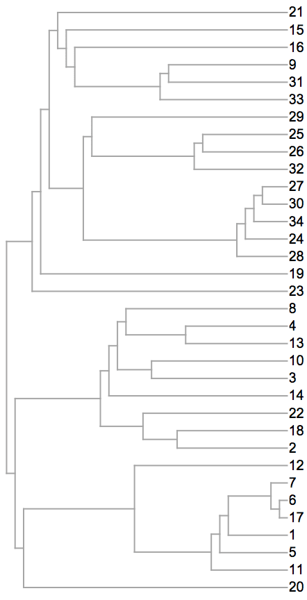
An Eulerian path passes through each edge of a graph precisely once. An Eulerian cycle is a closed Eulerian path: its starting vertex is the same as its ending vertex. Eulerian paths are also known as Eulerian trails.
Note: As of IGraph/M 0.5, the Eulerian path functions are still experimental.
?IGEulerianQ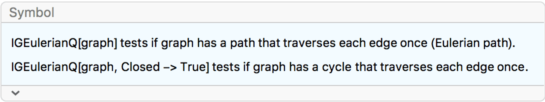
The following graph does not have an Eulerian path:
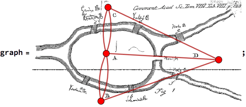
IGEulerianQ[graph]False
Removing the edge A <-> D makes it Eulerian:
IGEulerianQ@EdgeDelete[graph, "A" <-> "D"]True
But it will only have an Eulerian path, not an Eulerian cycle:
IGEulerianQ[
EdgeDelete[graph, "A" <-> "D"],
Closed -> True
]False
One possible path is the following:
IGEulerianPathVertices[EdgeDelete[graph, "A" <-> "D"]]{"B", "A", "B", "D", "C", "A", "C"}
?IGEulerianPath
?IGEulerianPathVertices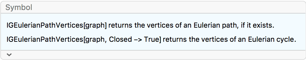
Find an Eulerian cycle through an icosidodecahedral graph:
g = GraphData["IcosidodecahedralGraph"];
cycle = IGEulerianPath[g, Closed -> True]{1 <-> 5, 5 <-> 7, 7 <-> 8, 6 <-> 8, 2 <-> 6, 2 <-> 16, 6 <-> 16, 6 <-> 30, 8 <-> 30, 8 <-> 14, 7 <-> 14, 7 <-> 29, 5 <-> 29, 5 <-> 15, 1 <-> 15, 1 <-> 18, 18 <-> 20, 11 <-> 20, 11 <-> 12, 3 <-> 12, 3 <-> 9, 9 <-> 15, 15 <-> 22, 9 <-> 22, 9 <-> 17, 3 <-> 17, 3 <-> 27, 12 <-> 27, 12 <-> 13, 4 <-> 13, 4 <-> 10, 10 <-> 16, 16 <-> 23, 14 <-> 23, 14 <-> 22, 22 <-> 23, 10 <-> 23, 10 <-> 17, 4 <-> 17, 4 <-> 28, 2 <-> 28, 2 <-> 19, 19 <-> 21, 11 <-> 21, 11 <-> 13, 13 <-> 28, 19 <-> 28, 19 <-> 26, 21 <-> 26, 20 <-> 21, 20 <-> 25, 24 <-> 25, 24 <-> 26, 26 <-> 30, 24 <-> 30, 24 <-> 29, 25 <-> 29, 18 <-> 25, 18 <-> 27, 1 <-> 27}
Visualize it using colour hues:
HighlightGraph[g,
MapIndexed[Style[#1, Hue[First[#2]/Length[cycle]]] &, cycle],
GraphStyle -> "ThickEdge"
]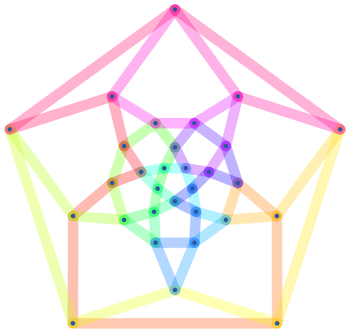
Direct the edges of the graph along the cycle:
Graph[
VertexList[g],
DirectedEdge @@@
Partition[IGEulerianPathVertices[g, Closed -> True], 2, 1],
EdgeStyle -> Arrowheads[Medium],
VertexCoordinates -> GraphEmbedding[g]
]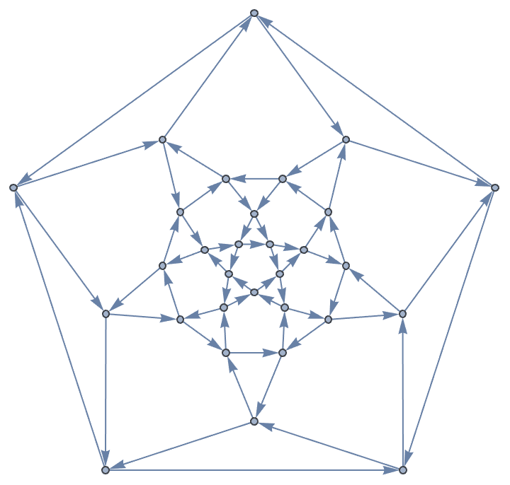
The graph colouring problem is assigning “colours” or “labels” to the vertices of a graph so that no two adjacent vertices will have the same colour. Similarly, edge colouring assigns colours to edges so that adjacent edges never have the same colour.
IGraph/M represents colours with the integers 1, 2, ….
Edge directions and self-loops are ignored.
?IGVertexColoring
?IGEdgeColoring
These function will find a colouring of the graph using a fast heuristic algorithm. The colouring may not be minimal. Edge directions are ignored.
Compute a vertex colouring of a Mycielski graph.
g = GraphData[{"Mycielski", 4}]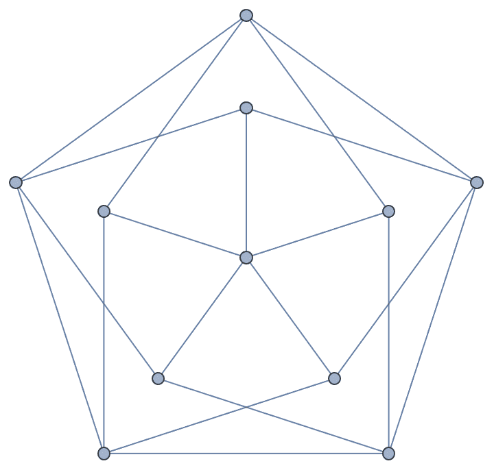
IGVertexColoring returns a list of integers, each
representing the colour of the vertex that is in the same position in
the vertex list.
IGVertexColoring[g]{4, 3, 1, 1, 3, 1, 2, 2, 2, 2, 2}
Associate the colours with vertex names.
AssociationThread[VertexList[g], IGVertexColoring[g]]<|1 -> 4, 2 -> 3, 3 -> 1, 4 -> 1, 5 -> 3, 6 -> 1, 7 -> 2, 8 -> 2, 9 -> 2, 10 -> 2, 11 -> 2|>
Visualize the colours using IGraph/M’s property mapping functionality. See the Property handling functions documentation section for more information.
Graph[g, VertexSize -> 1/3, EdgeStyle -> Gray] //
IGVertexMap[ColorData[97], VertexStyle -> IGVertexColoring]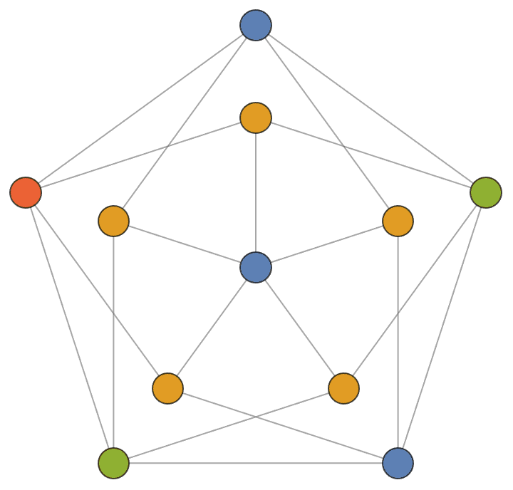
Visualize an edge colouring of the same graph.
Graph[g, GraphStyle -> "ThickEdge", EdgeStyle -> Opacity[0.7],
VertexStyle -> Black] //
IGEdgeMap[ColorData[106], EdgeStyle -> IGEdgeColoring]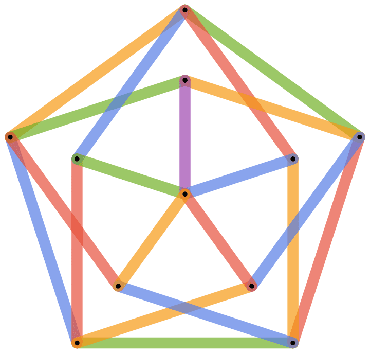
Compute a checkerboard-like colouring of a three-dimensional grid graph.
IGVertexMap[ColorData[97], VertexStyle -> IGVertexColoring,
Graph3D@GridGraph[{4, 4, 4}, VertexSize -> 0.8]]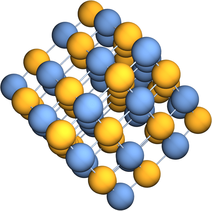
Compute a colouring of a Voronoi mesh.
mesh = VoronoiMesh[RandomReal[1, {20, 2}]]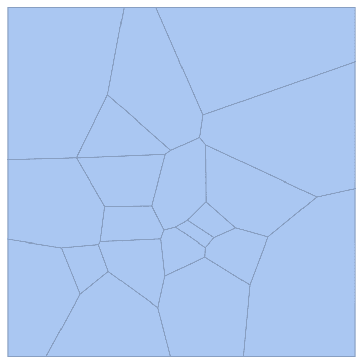
col = IGVertexColoring@IGMeshCellAdjacencyGraph[mesh, 2]{2, 5, 4, 2, 1, 1, 2, 2, 4, 1, 3, 1, 2, 3, 3, 4, 2, 1, 3, 1}
SetProperty[{mesh, {2, All}}, MeshCellStyle -> ColorData[97] /@ col]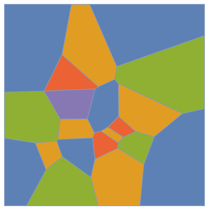
Compute a colouring of the map of African countries.
countries = CountryData["Africa"];
borderingQ[c1_, c2_] := MemberQ[c1["BorderingCountries"], c2]
graph = RelationGraph[borderingQ, countries];GeoGraphics@
MapThread[{GeoStyling[{Opacity[0.5], #2}],
Polygon[#1]} &, {countries,
ColorData[97] /@ IGVertexColoring[graph]}]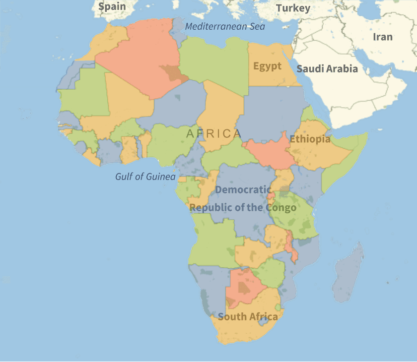
?IGKVertexColoring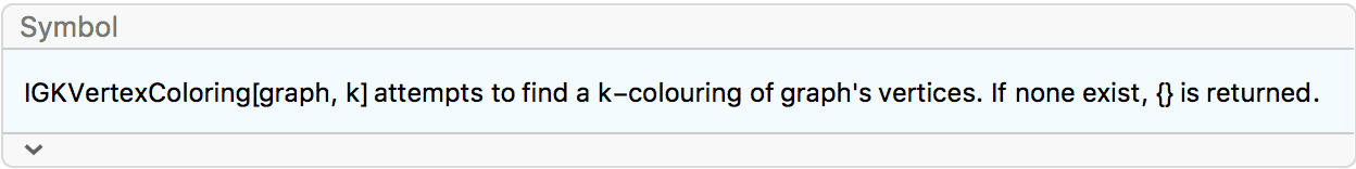
?IGKEdgeColoring
These functions find a colouring with \(k\) or fewer colours. They work by
transforming the colouring into a satisfiability problem and using
SatisfiabilityInstances.
The available option values are:
![]() forces the given vertices to distinct and increasing colours. Normally,
the vertices of a clique are given (which require as many colours as the
size of the clique). The main purpose of this option is to reduce the
number of redundant solutions of the equivalent SAT problem, and thus
improve performance. When using edge colouring functions, a set of edges
should be passed.
forces the given vertices to distinct and increasing colours. Normally,
the vertices of a clique are given (which require as many colours as the
size of the clique). The main purpose of this option is to reduce the
number of redundant solutions of the equivalent SAT problem, and thus
improve performance. When using edge colouring functions, a set of edges
should be passed.
"ForcedColoring" -> "MaxDegreeClique" attempts to
find a clique containing a maximum degree vertex, and forces colours on
the clique members. On hard problems it may perform orders of magnitude
better than "ForcedColoring" -> None.
"ForcedColoring" -> "LargestClique" finds a
largest clique, and forces colours on the clique members.
"ForcedColoring" -> None does not force any
colours. It is usually the fastest choice for easy problems.
The default setting for "ForcedColoring" is
"MaxDegreeClique".
The Moser spindle is not 3-colourable, so no solution is returned.
moser = GraphData["MoserSpindle"];IGKVertexColoring[moser, 3]{}
Find a 4-colouring of the Moser spindle …
IGKVertexColoring[moser, 4]{{4, 1, 3, 1, 3, 2, 2}}
… and visualize it.
Graph[moser, GraphStyle -> "BasicBlack", VertexSize -> Large] //
IGVertexMap[ColorData[112],
VertexStyle -> (First@IGKVertexColoring[#, 4] &)]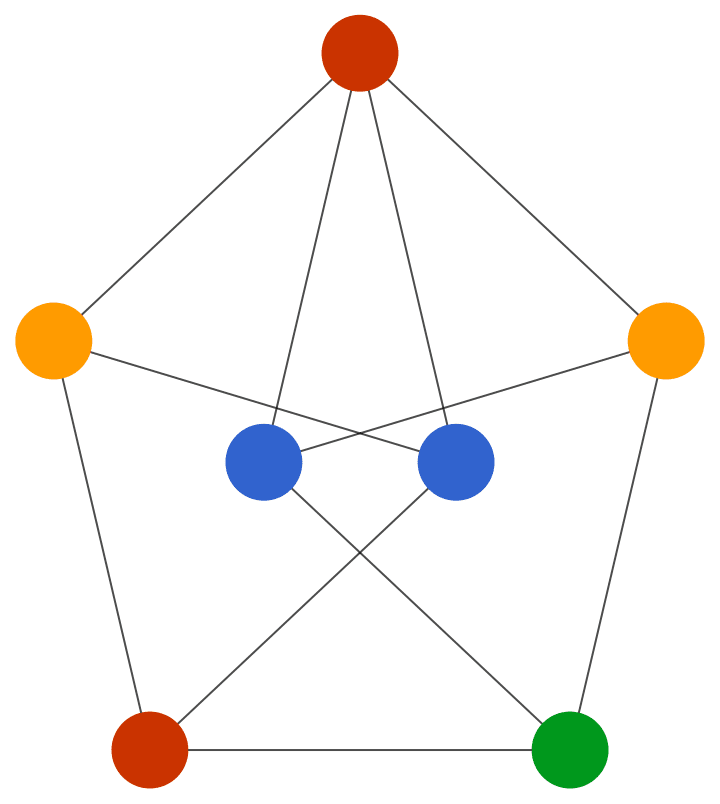
Find a 4-edge-colouring of the Petersen graph.
PetersenGraph[GraphStyle -> "ThickEdge", EdgeStyle -> Opacity[2/3]] //
IGEdgeMap[ColorData[112],
EdgeStyle -> (First@IGKEdgeColoring[#, 4] &)]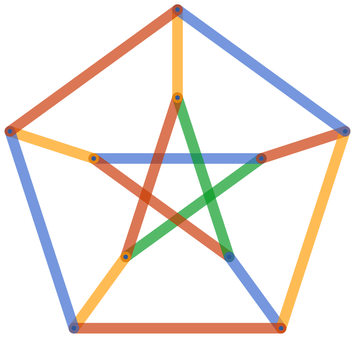
The following examples illustrate the use of the
"ForcedColoring" option. The 6th order Mycielski graph has
chromatic number 6. A 6-colouring is easily found even with
"ForcedColoring" -> None.
g = GraphData[{"Mycielski", 6}];IGKVertexColoring[g, 6, "ForcedColoring" -> None] // Timing{0.010348, {{6, 4, 5, 5, 4, 4, 1, 1, 1, 1, 1, 3, 3, 3, 3, 3, 3, 3, 3, 3, 3, 3, 1, 2, 2, 2, 2, 2, 2, 2, 2, 2, 2, 2, 2, 2, 2, 2, 2, 2, 2, 2, 2, 2, 2, 2, 1}}}
However, showing that the graph is not 5-colourable takes considerably longer.
TimeConstrained[IGKVertexColoring[g, 5, "ForcedColoring" -> None], 5]$Aborted
Forcing colours in the appropriate way reduces the computation time significantly.
IGKVertexColoring[g, 5,
"ForcedColoring" -> "MaxDegreeClique"] // Timing{0.311691, {}}
?IGMinimumVertexColoring
?IGMinimumEdgeColoring
IGMinimumVertexColoring and
IGMinimumEdgeColoring find minimum colourings of graphs,
i.e. they find a colouring with the fewest possible number of colours.
The current implementation tries successively larger \(k\)-colourings until it is successful.
IGMinimumVertexColoring and
IGMinimumEdgeColoring can use the same
"ForcedColoring" option values as
IGKVertexColoring and IGKEdgeColoring.
WheelGraph[7, GraphStyle -> "BasicBlack", VertexSize -> Large] //
IGVertexMap[ColorData[97], VertexStyle -> IGMinimumVertexColoring]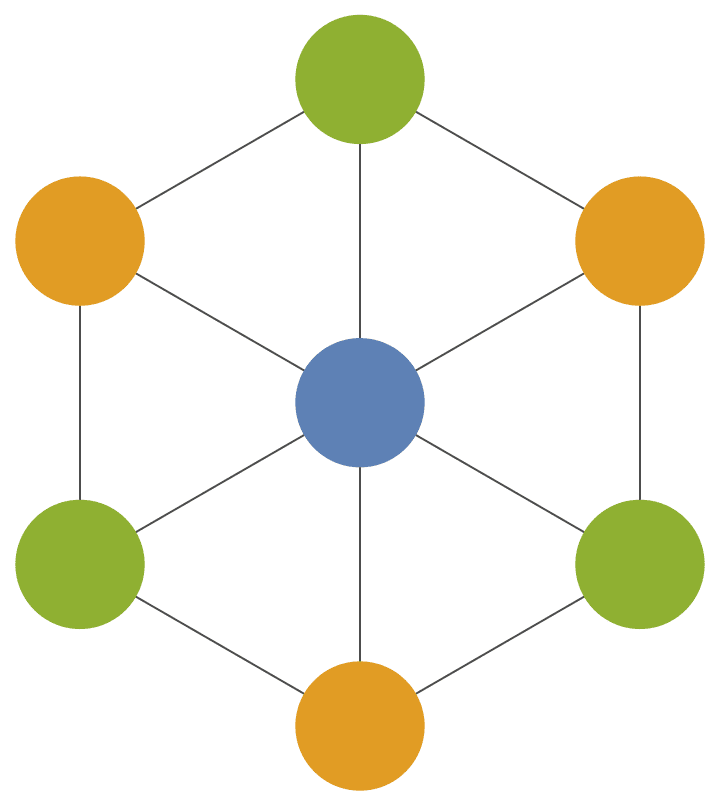
Find a colouring of a large graph.
IGMinimumVertexColoring@RandomGraph[{100, 400}]{3, 1, 1, 3, 2, 2, 2, 1, 4, 1, 2, 4, 3, 4, 4, 4, 1, 1, 1, 2, 4, 4, 3, \ 1, 2, 1, 4, 2, 4, 3, 3, 2, 3, 3, 3, 2, 4, 1, 3, 3, 1, 3, 2, 4, 4, 2, \ 1, 2, 2, 4, 3, 4, 4, 2, 4, 3, 3, 2, 1, 1, 4, 2, 3, 4, 3, 1, 1, 2, 1, \ 3, 4, 1, 1, 2, 2, 2, 1, 2, 2, 3, 4, 3, 1, 2, 1, 3, 2, 1, 3, 2, 4, 3, \ 4, 2, 3, 4, 3, 3, 4, 4}
Implement a multipartite graph layout: vertex colouring is equivalent
to partitioning the vertices of the graph into groups such that all
connections run between different groups, and never within the same
group. The colours can be thought of as the indices of groups.
IGMembershipToPartitions can be used to convert from a
group-index (i.e. membership) representation to a partition
representation.
multipartiteLayout[g_?GraphQ, separation : _?NumericQ : 1.5,
opt : OptionsPattern[]] :=
Module[{n, partitions, partitionSizes, vertexCoordinates},
partitions = IGMembershipToPartitions[g]@IGMinimumVertexColoring[g];
partitionSizes = Length /@ partitions;
n = Length[partitions];
vertexCoordinates =
With[{hl = N@Sin[Pi/n],
ir = separation If[n == 2, 1/2, N@Cos[Pi/n]]},
Catenate@Table[
RotationTransform[2 Pi/n k][{#, ir} & /@
Subdivide[-hl, hl, partitionSizes[[k]] - 1]],
{k, 1, n}
]
];
IGReorderVertices[Catenate[partitions], g,
VertexCoordinates -> vertexCoordinates, opt]
];Lay out a bipartite graph.
g = IGBipartiteGameGNM[10, 10, 30];
multipartiteLayout[g]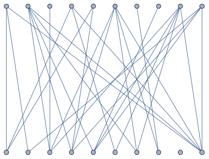
Lay out multipartite graphs.
g = RandomGraph[{40, 40}];
multipartiteLayout[g]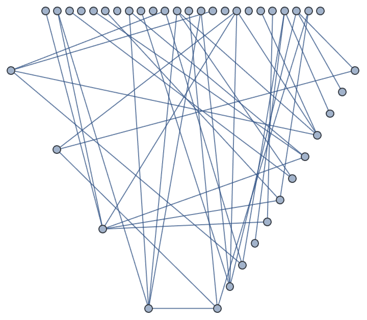
g = RandomGraph[{40, 160}];
multipartiteLayout[g, GraphStyle -> "BasicBlack",
EdgeStyle -> Opacity[0.2]]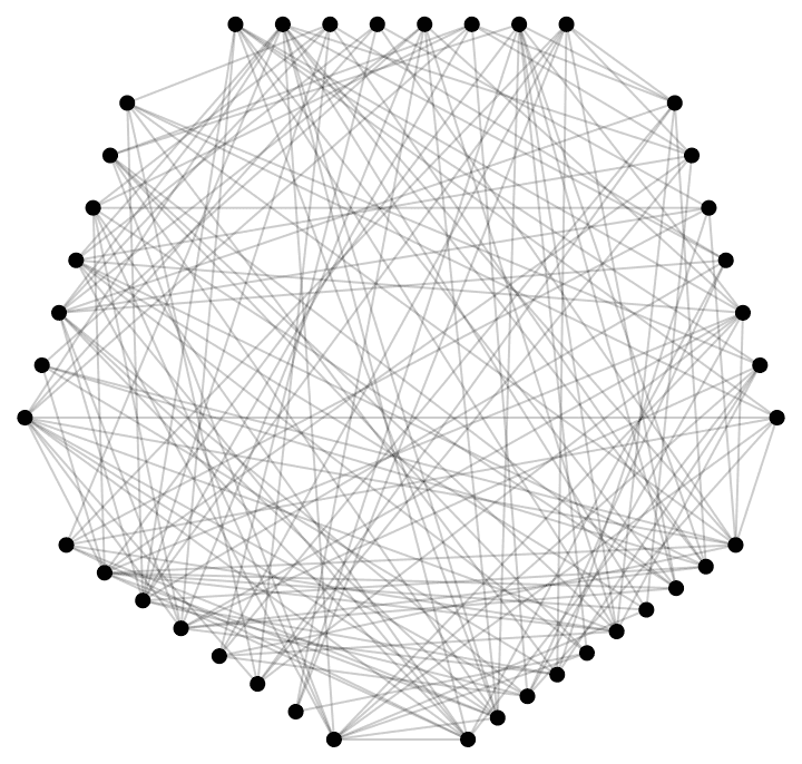
Compute a minimum colouring of a triangulation. It can be shown, e.g. based on Brooks’s theorem, that any triangulation of a polygon is 3-colourable.
mesh = DelaunayMesh[RandomReal[1, {20, 2}],
MeshCellStyle -> {1 -> Black}];
col = IGMinimumVertexColoring@IGMeshCellAdjacencyGraph[mesh, 2];
SetProperty[{mesh, {2, All}}, MeshCellStyle -> ColorData[97] /@ col]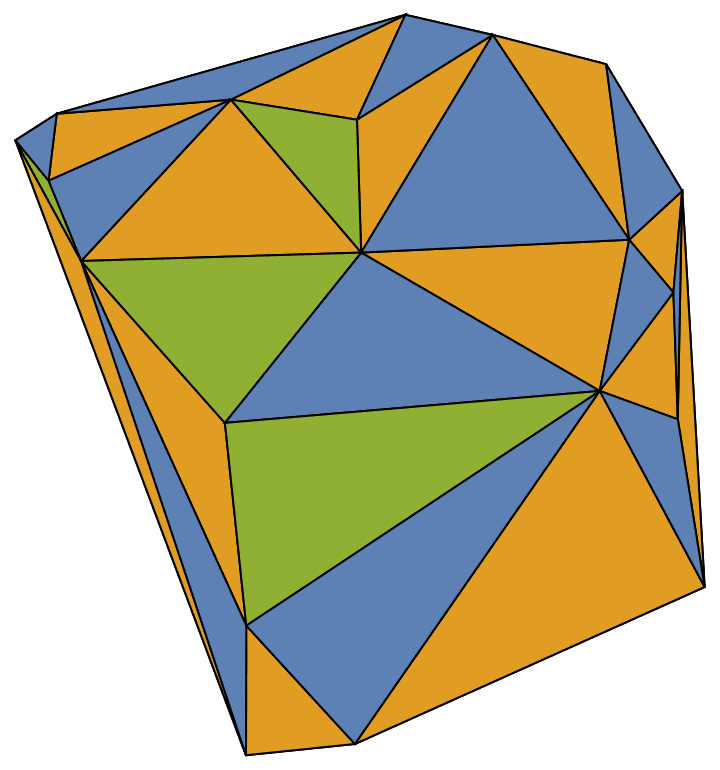
Find a minimum edge colouring of a graph.
Graph[
GraphData["SixteenCellGraph"],
GraphStyle -> "ThickEdge", EdgeStyle -> Opacity[2/3]
] //
IGEdgeMap[
ColorData[104],
EdgeStyle -> IGMinimumEdgeColoring
]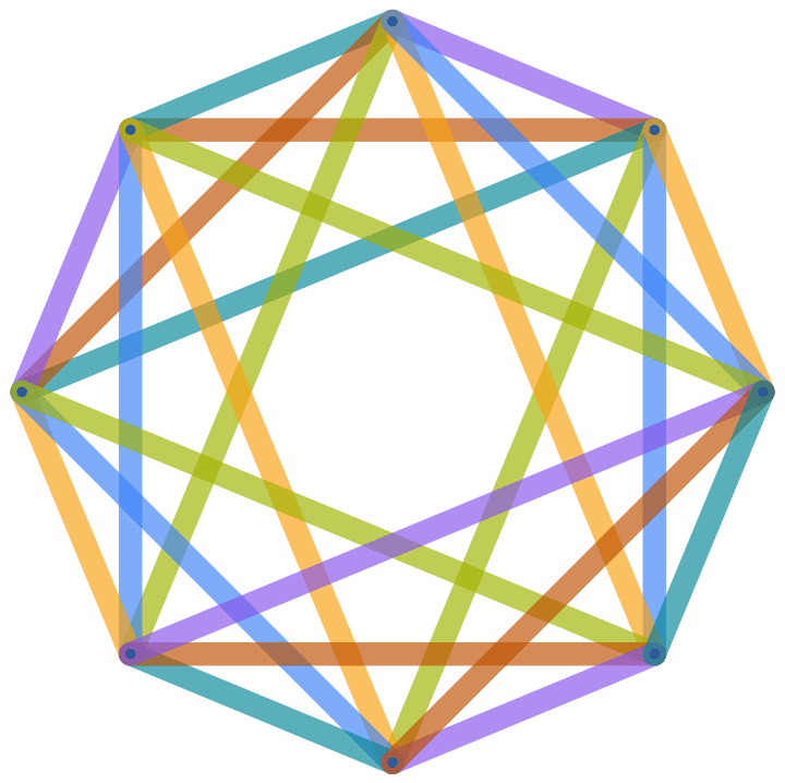
?IGChromaticNumber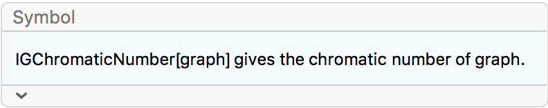
?IGChromaticIndex
The chromatic number of a graph is the smallest number of colours needed to colour its vertices. The chromatic index, or edge chromatic number, is the smallest number of colours needed to colour its edges.
Find the chromatic number and chromatic index of a graph.
g = GraphData["IcosahedralGraph"]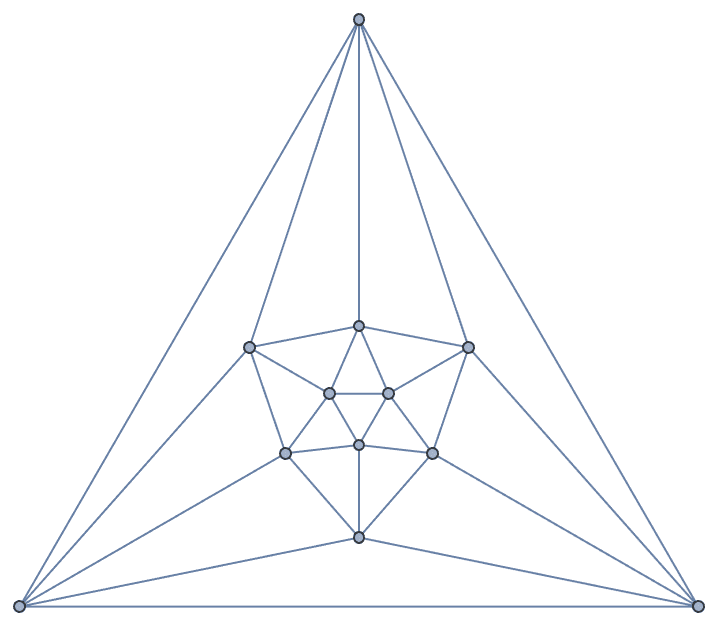
{IGChromaticNumber[g], IGChromaticIndex[g]}{4, 5}
The implementation of IGChromaticNumber and
IGChromaticIndex is effectively the following:
{Max@IGMinimumVertexColoring[g], Max@IGMinimumEdgeColoring[g]}{4, 5}
?IGPerfectQ
IGPerfectQ tests if a graph is perfect. The clique
number and the chromatic number is the same for every induced subgraph
of a perfect graph.
The current implementation of IGPerfectQ uses the strong
perfect graph theorem: it checks that neither the graph nor its
complement have a graph hole of odd length.
g = GraphData[{"GeneralizedQuadrangle", {2, 1}}]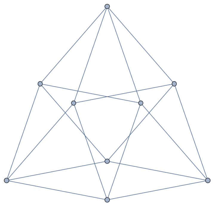
IGPerfectQ[g]True
The clique number and the chromatic number is the same for every induced subgraph.
AllTrue[
Subgraph[g, #] & /@ Subsets@VertexList[g],
IGCliqueNumber[#] == IGChromaticNumber[#] &
]True
?IGVertexColoringQ
IGVertexColoringQ checks whether neighbouring vertices
of a graph are assigned different colours.
The colours may be given as a list, with the same ordering as
VertexList[graph].
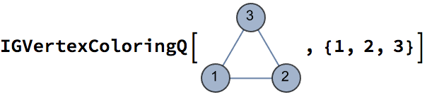
True

False
The colours may also be given as an association from vertices to colours.
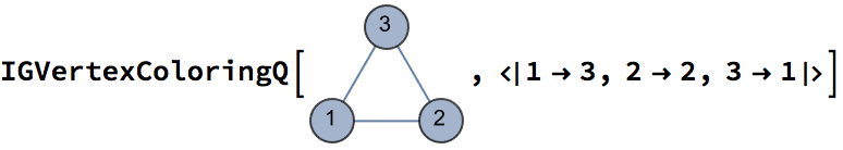
True
Any expression may be used for the colours, not only integers.
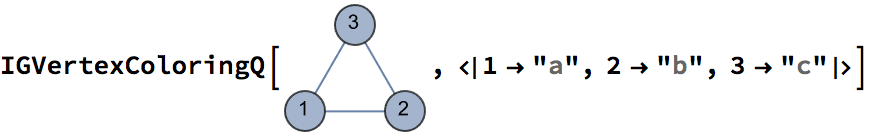
True
?IGRandomWalk
IGRandomWalk[] takes a random walk over a directed or
undirected graph. If the graph is weighted, the next edge to traverse is
selected with probability proportional to its weight.
The available options are:
EdgeWeight can be used to override the existing weights
of the graph. EdgeWeight -> None will ignore any
existing weights.Traversing self-loops in different directions is considered as distinct probabilities in an undirected graph. Thus vertices 1 and 3 are visited more often in the below graphs than vertex 2:
g = Graph[{1 <-> 1, 1 <-> 2,
2 <-> 3, 3 <-> 3},
VertexLabels -> "Name"]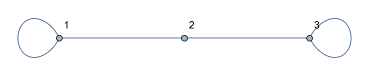
IGRandomWalk[g, 1, 100000] // Counts // KeySort<|1 -> 37453, 2 -> 25082, 3 -> 37465|>
This is consistent with their degrees:
VertexDegree[g]{3, 2, 3}
Convert the graph to a directed version to traverse self-loops only in one direction.
dg = DirectedGraph[g]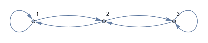
{VertexOutDegree[dg], VertexInDegree[dg]}{{2, 2, 2}, {2, 2, 2}}
IGRandomWalk[dg, 1, 100000] // Counts // KeySort<|1 -> 33345, 2 -> 33317, 3 -> 33338|>
If the walker gets stuck, a list shorter than steps will
be returned. This may happen in a non-connected directed graph, or in a
single-vertex graph component.
IGRandomWalk[IGEmptyGraph[1], 1, 10]{1}
IGRandomWalk[Graph[{1 -> 2}], 1, 10]{1, 2}
How much time does a random walker spend on each node of a network?
g = IGBarabasiAlbertGame[50, 2, DirectedEdges -> False]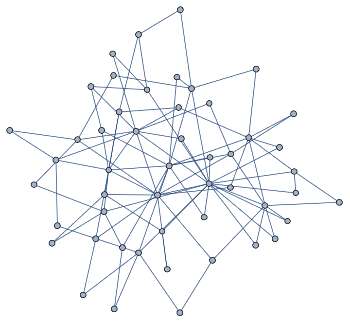
counts =
Counts@IGRandomWalk[g, First@VertexList[g], 10000] /@ VertexList[g]{591, 550, 411, 906, 545, 198, 261, 411, 242, 420, 151, 247, 215, \ 171, 280, 113, 88, 216, 277, 133, 115, 158, 103, 99, 143, 93, 100, \ 123, 254, 188, 155, 175, 89, 113, 123, 96, 100, 87, 141, 81, 88, 93, \ 98, 111, 106, 115, 101, 96, 125, 105}
The exact answer can be computed as the leading eigenvector of the process’s stochastic matrix:

Compare the exact answer with a finite sample:
![]()
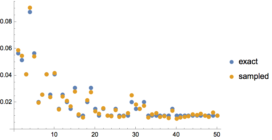
Random walk on a square grid.
grid = IGSquareLattice[{50, 50}];
counts = Counts@IGRandomWalk[grid, 1, 5000];
Graph[grid,
VertexStyle ->
Prepend[
Normal[ColorData["SolarColors"] /@ Normalize[counts, Max]],
Black (* colour of unvisited nodes, i.e. default colour *)
],
EdgeShapeFunction -> None,
Background -> Black
]
The fraction of nodes reached after \(n\) steps on a grid and a comparable random regular graph.
nodesReached[graph_] :=
Length@Union@IGRandomWalk[graph, 1, VertexCount[graph]]/
VertexCount[graph]grid = IGSquareLattice[{50, 50}, "Periodic" -> True];
regular = IGKRegularGame[50^2, 4];Table[
{nodesReached[grid], nodesReached[regular]},
{5000}
] // Transpose // Histogram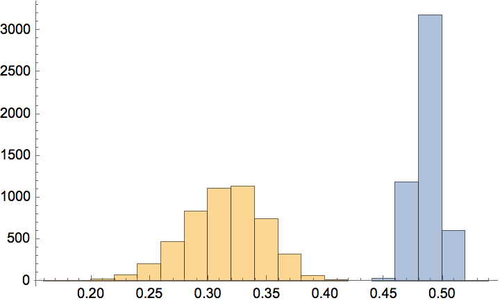
Generate random spanning trees using loop erased random walks.
randomSpanningTree[graph_?GraphQ] :=
Module[{visited = <||>, i = 2, k = 1,
batchSize = 2 VertexCount[graph], walk},
walk =
IGRandomWalk[graph, RandomChoice@VertexList[graph], batchSize];
visited[walk[[1]]] = True;
While[k < VertexCount[graph],
(*
register a traversed edge only when it leads to a yet unvisited \
vertex *)
If[! TrueQ[visited[walk[[i]]]],
Sow[walk[[i - 1]] <-> walk[[i]]];
visited[walk[[i]]] = True;
k++
];
i++;
(* if the walk has not yet visited all vertices, keep walking *)
If[i > Length[walk],
walk =
Join[walk, Rest@IGRandomWalk[graph, Last[walk], batchSize]]
];
] // Reap // Last // First
]By taking random spanning trees of spatially embedded planar graphs, we can generate mazes.
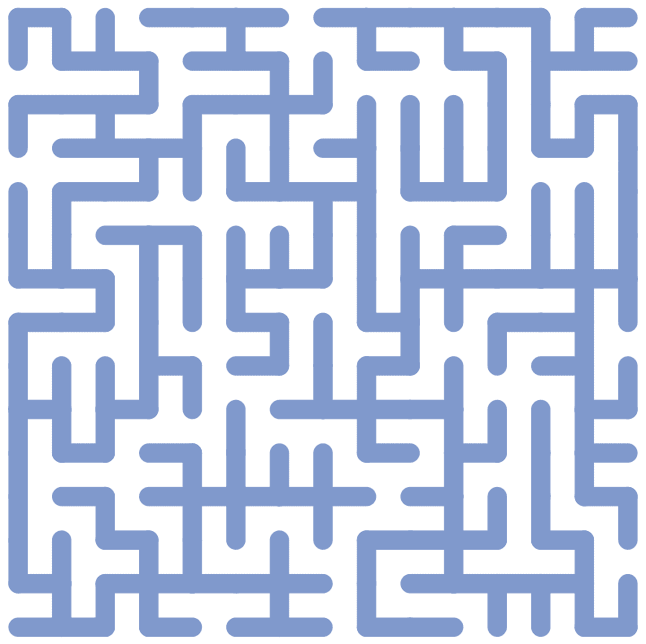
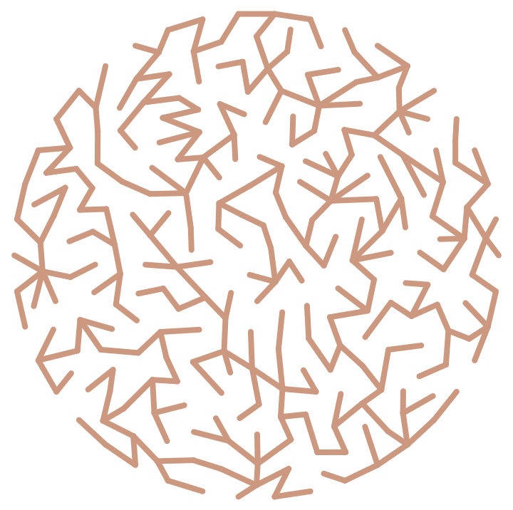
Take a sample of a large graph using a random walk. The following graph is too large to easily visualize, but visualizing a random-walk-based sample immediately shows signs of a community structure.
g = ExampleData[{"NetworkGraph", "AstrophysicsCollaborations"}];
{VertexCount[g], VertexCount@IGGiantComponent[g]}{16706, 14845}
Subgraph[g,
IGRandomWalk[g, RandomChoice@VertexList@IGGiantComponent[g], 200]]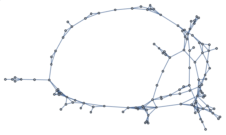
CommunityGraphPlot[%]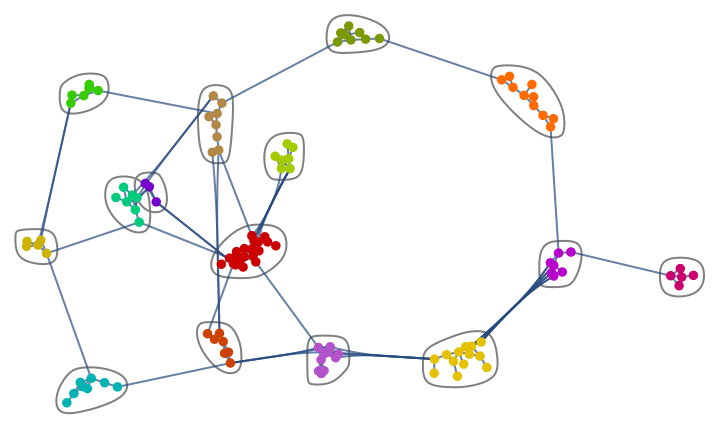
?IGRandomEdgeWalk
?IGRandomEdgeIndexWalk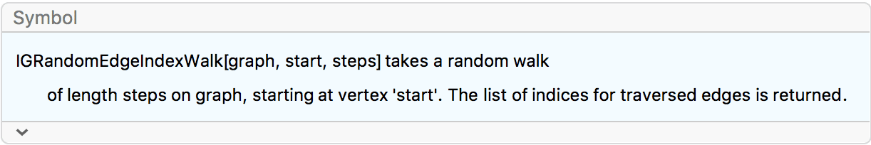
IGRandomEdgeWalk takes a random walk on a graph and
returns the list of traversed edges. If the graph is weighted, the next
edge to traverse is selected with probability proportional to its
weight.
The available options are:
EdgeWeight can be used to override the existing weights
of the graph. EdgeWeight -> None will ignore any
existing weights.Take a random walk on a De Bruijn graph, and retrieve the traversed edges.
g = IGDeBruijnGraph[3, 3];
IGRandomEdgeWalk[g, RandomChoice@VertexList[g], 20]{13 \[DirectedEdge] 11, 11 \[DirectedEdge] 6, 6 \[DirectedEdge] 16, 16 \[DirectedEdge] 21, 21 \[DirectedEdge] 9, 9 \[DirectedEdge] 25, 25 \[DirectedEdge] 21, 21 \[DirectedEdge] 7, 7 \[DirectedEdge] 20, 20 \[DirectedEdge] 6, 6 \[DirectedEdge] 16, 16 \[DirectedEdge] 19, 19 \[DirectedEdge] 1, 1 \[DirectedEdge] 3, 3 \[DirectedEdge] 7, 7 \[DirectedEdge] 19, 19 \[DirectedEdge] 2, 2 \[DirectedEdge] 4, 4 \[DirectedEdge] 11, 11 \[DirectedEdge] 4}
IGRandomEdgeIndexWalk returns the list of indices of the
traversed edges instead. This makes it useful for working with
multigraphs, as it allows distinguishing between parallel edges.
As an example application, let us consider the following set of affine transformations:
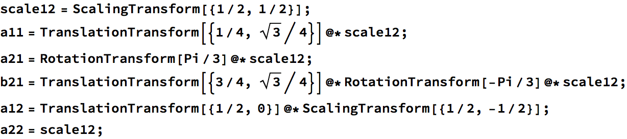
trafos = {a11, a21, b21, a12, a22};Let us visualize them by showing an initial (black) triangle and its (red) transformation.
![]()
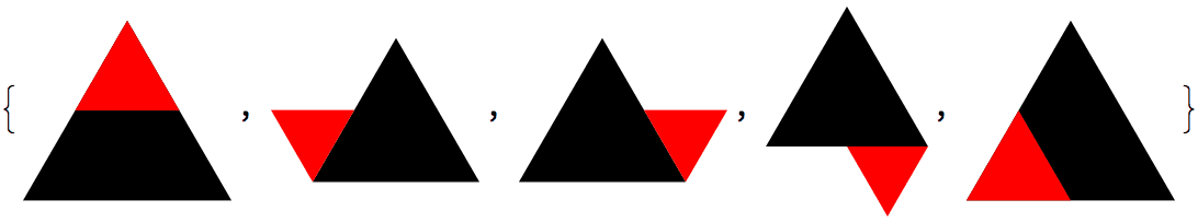
These transformations describe the mutual self-similarity structure of two fractal curves, according to the following directed graph. Each edge of the graph corresponds to a transformation.
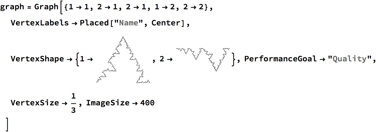
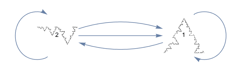
Let us compute a random walk on this graph, and iteratively apply
transformations to the point {0, 0} according to the
traversed edges.
walk = IGRandomEdgeIndexWalk[graph, 1, 20000];
pts = Rest@FoldList[#2[#1] &, {0., 0.}, trafos[[walk]]];The resulting list of points will approximate the union of the two fractal curves.
Image@Graphics[{AbsolutePointSize[1], Point[pts]}]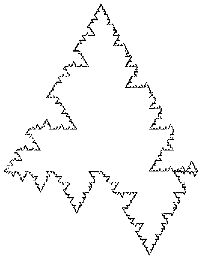
The two curves can be separated by filtering points according to
which graph vertex the corresponding directed edge targets. For example,
if the point was generated by a transformation corresponding to
1 \[DirectedEdge] 2, it will belong to curve
2.
targets = Last /@ EdgeList[graph]{1, 1, 1, 2, 2}
Image@Graphics[{AbsolutePointSize[1],
Point@Pick[pts, targets[[walk]], 1]}]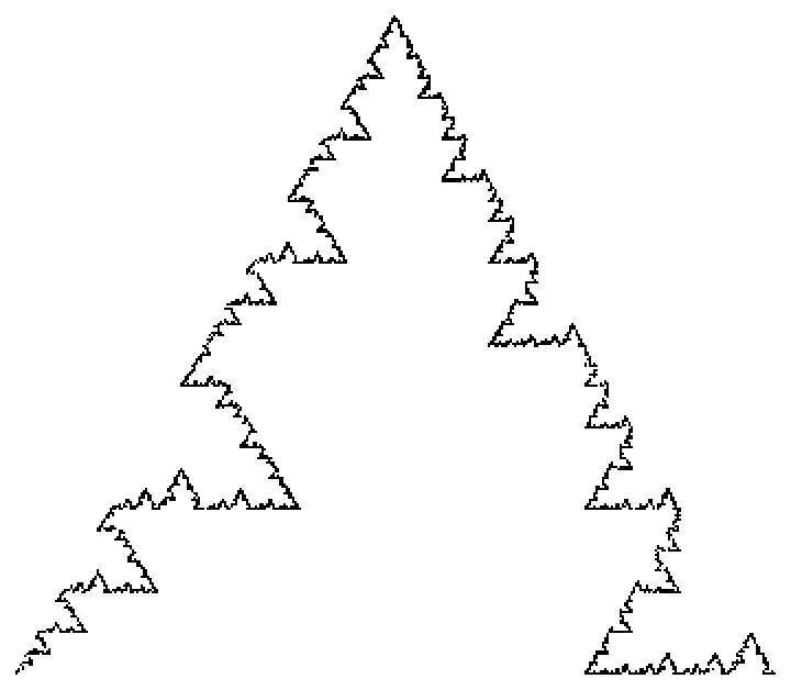
Image@Graphics[{AbsolutePointSize[1],
Point@Pick[pts, targets[[walk]], 2]}]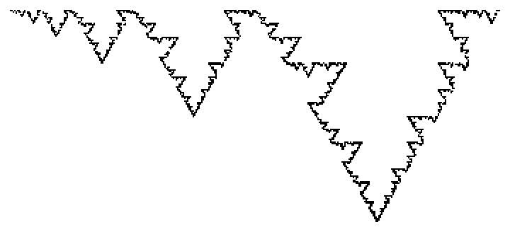
The technique described here is taken from “Generating self-affine tiles and their boundaries” by Mark McClure.
?IGSIRProcess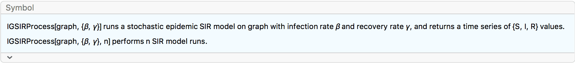
IGSIRProcess simulates a stochastic version of the well
known SIR model of disease spreading. In this model, each node of the
network may be in one of three states: susceptible, infected or
recovered, denoted by \(S\), \(I\) and \(R\), respectively. A susceptible node with
\(k\) infected neighbours becomes
infected with rate \(k \beta\), while
an infected node recovers with rate \(\gamma\). At the start of the simulation, a
random node is chosen to be infected. The simulation runs until no more
infected nodes are left.
When performing a single simulation, IGSIRProcess
returns a TimeSeries
expression of {s, i, r} values. When multiple runs are
requested, the resulting time series are combined into a TemporalData
expression.
g = IGWattsStrogatzGame[100, 0.05];Perform a single SIR simulation:
ts = IGSIRProcess[g, {5, 1}]![]()
Plot the results with a legend:
ListLinePlot[ts, PlotLegends -> ts["ComponentNames"]]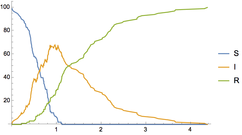
Plot only the number of infected nodes:
(* In Mathematica 12.0 and later,
ts["PathComponent", "I"] can also be used. *)
ListLinePlot[ts["PathComponent", 2],
AxesLabel -> {"time", "infected"}, PlotStyle -> ColorData[97][2]]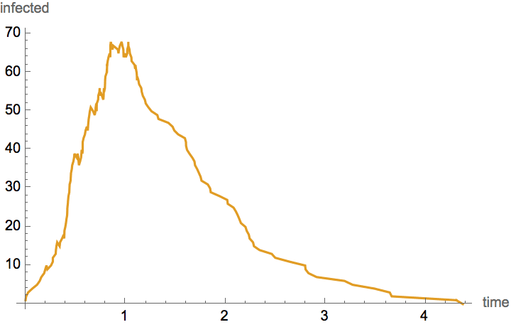
Find the number of susceptible, infected and recovered nodes at a specific time point:
ts[1.0]{6., 65., 29.}
The ResamplingMethod of the TimeSeries object is set to 0th order interpolation, therefore the last value is used beyond the last available time point.
ts[10]![]()
{0., 0., 100.}
Perform 100 simulations simultaneously:
td = IGSIRProcess[g, {5, 1}, 100]![]()
Plot the median number of susceptible, infected and recovered nodes:
Show[
ListLinePlot[#, PlotStyle -> GrayLevel[0, 0.1],
PlotRange -> {0, VertexCount[g]}],
Quiet@Plot[Median[#[t]], {t, 0, 4}, PlotStyle -> Red]
] & /@ td["PathComponents"] // GraphicsColumn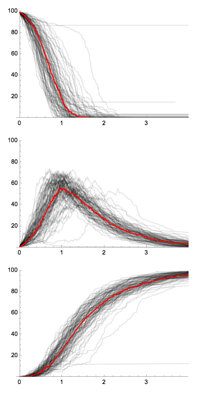
The sum of the three components, \(S+I+R\), always equals the total number of graph nodes.
First@Normal@Total[td["PathComponents"]] // Short![]()
In the next example, we compare epidemic spreading on a periodic grid, i.e. a network that only has spatially local connections, with a rewired version of the same network which also includes long range links. We rewire 5% of links while ensuring that the graph stays connected.
g1 = IGSquareLattice[{30, 30}, "Periodic" -> True];
g2 = IGTryUntil[IGConnectedQ][IGRewireEdges[g1, 0.05]];Generate 1000 simulations for each network.
r1 = IGSIRProcess[g1, {1, 1}, 1000];
r2 = IGSIRProcess[g2, {1, 1}, 1000];Plot the histogram of the total duration of the epidemic.
Histogram[{r1["LastTimes"], r2["LastTimes"]},
ChartLegends -> {"grid", "rewired"}]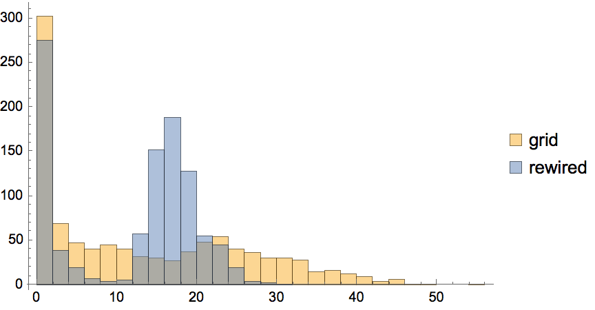
Plot the fraction of recovered nodes at the end of the epidemic.
tmax = Max[r1["MaximumTime"], r2["MaximumTime"]];
Histogram[
{r1["PathComponent", 3]["SliceData", tmax]/VertexCount[g1],
r2["PathComponent", 3]["SliceData", tmax]/VertexCount[g2]} // Quiet,
{0, 1, 0.02},
ChartLegends -> {"grid", "rewired"}
]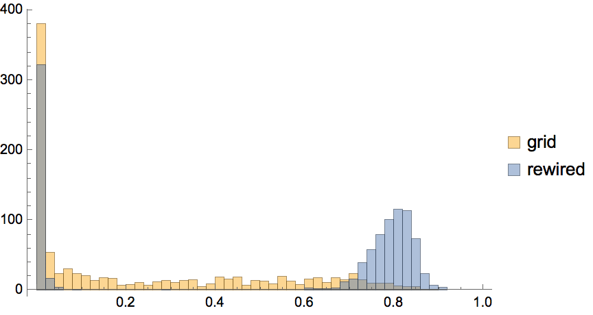
A graph is said to be planar if it can be drawn in the plane without edge crossings.
A useful concept when working with planar graphs is their combinatorial embedding. A combinatorial embedding of a graph is a counter-clockwise ordering of the incident edges around each vertex. IGraph/M represents combinatorial embeddings as associations from vertices to an ordering of their neighbours. Currently, only embeddings of simple graphs are supported.
Some of the planar graph functionality makes use of the LEMON Graph Library.
?IGPlanarQ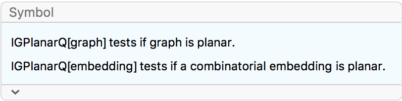
IGPlanarQ[graph] checks if a graph is planar using the
Boyer–Myrvold algorithm.
IGPlanarQ@GraphData[{"Apollonian", 6}]True
IGPlanarQ@CompleteGraph[5]False
IGPlanarQ[embedding] checks if a combinatorial embedding
is planar. The following are both embeddings of the \(K_4\) complete graph. However, only the
first one is planar.
emb1 = <|1 -> {2, 3, 4}, 2 -> {1, 4, 3}, 3 -> {2, 4, 1},
4 -> {3, 2, 1}|>;
emb2 = <|1 -> {2, 4, 3}, 2 -> {4, 3, 1}, 3 -> {1, 2, 4},
4 -> {3, 1, 2}|>;IGPlanarQ /@ {emb1, emb2}{True, False}
The second embedding generates only 2 faces instead of 4, which can be embedded on a torus, but not in the plane (or on a sphere).
Length /@ IGFaces /@ {emb1, emb2}{4, 2}
Unlike the built-in PlanarGraphQ, IGPlanarQ
considers the null graph to be planar.
{IGPlanarQ@IGEmptyGraph[], PlanarGraphQ@IGEmptyGraph[]}{True, True}
?IGMaximalPlanarQ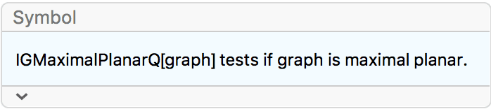
A simple graph is maximal planar if no new edges can be added to it without breaking planarity. Maximal planar graphs are sometimes called triangulated graphs or triangulations.
The 3-cycle is maximal planar.
IGMaximalPlanarQ[CycleGraph[3]]True
The 4-cycle is not because a chord can be added to it without breaking planarity.
IGMaximalPlanarQ[CycleGraph[4]]False
IGPlanarQ[EdgeAdd[CycleGraph[4], 1 <-> 3]]True
Apollonian graphs are maximal planar.
g = GraphData[{"Apollonian", 2}]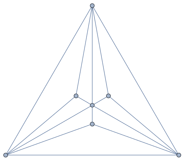
IGMaximalPlanarQ[g]True
All faces of a maximal planar graph are triangles.
Length /@ IGFaces[g]{3, 3, 3, 3, 3, 3, 3, 3, 3, 3}
Therefore the edge count \(E\) and the face count \(F\) of a maximal planar graph on more than 2 vertices satisfy \(2E=3F\). Each edge is incident to two faces and each face is incident to three edges.
{2 EdgeCount[g], 3 Length@IGFaces[g]}{30, 30}
?IGOuterplanarQ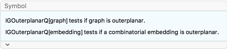
IGOuterplanarQ[graph] checks if a graph is outerplanar,
i.e. if it can be drawn in the plane without edge crossings and with all
vertices being on the outer face.
Outerplanar graphs are also called circular planar. They can be drawn
without edge crossings and all vertices on a circle. See the
documentation of IGOuterplanarEmbedding for an example.
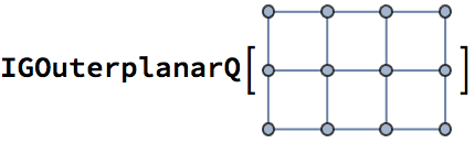
False
![]()
True
IGOuterplanarQ[embedding] checks if a combinatorial
embedding is outerplanar. Not all planar embeddings of an outerplanar
graph are also outerplanar embeddings.
Consider the following outerplanar graph …
g = IGShorthand["0-1-2-3-4-2,1-4"]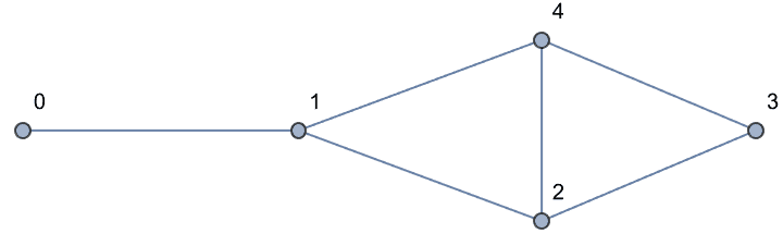
IGOuterplanarQ[g]True
… and two of its embeddings:
emb1 = <|0 -> {1}, 1 -> {2, 0, 4}, 2 -> {1, 3, 4}, 3 -> {2, 4},
4 -> {3, 1, 2}|>;
emb2 = <|0 -> {1}, 1 -> {0, 2, 4}, 2 -> {1, 3, 4}, 3 -> {2, 4},
4 -> {3, 1, 2}|>;They are both planar, but only the second one is outerplanar.
IGPlanarQ /@ {emb1, emb2}{True, True}
IGOuterplanarQ /@ {emb1, emb2}{False, True}
Graph[g, VertexCoordinates -> IGEmbeddingToCoordinates[#]] & /@ {emb1,
emb2}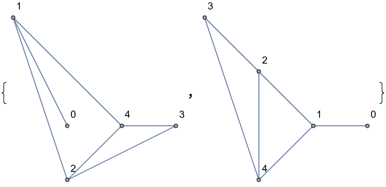
?IGKuratowskiEdges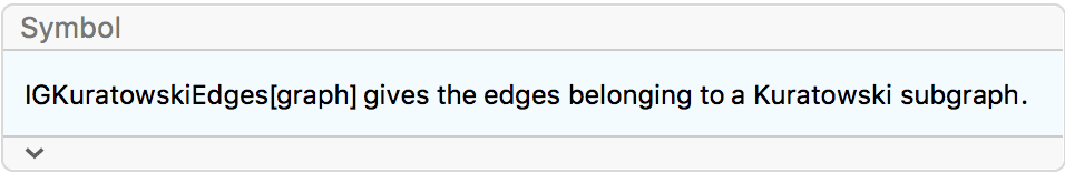
IGKuratowskiEdges finds a Kuratowski subgraph of a
non-planar graph. The subgraph is returned as a set of edges. If the
graph is planar, {} is returned.
According to Kuratowski’s theorem, any non-planar graph contains a subgraph homeomorphic to the \(K_5\) complete graph or the \(K_{3,3}\) complete bipartite graph. This is called a Kuratowski subgraph.
Generate a random graph, which is non-planar with high probability.
g = RandomGraph[{20, 40}]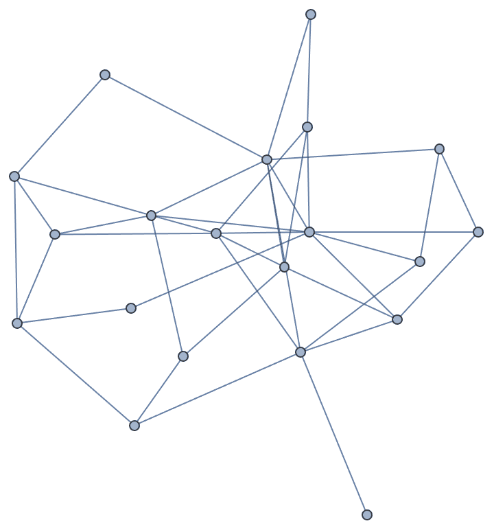
IGPlanarQ[g]False
Compute a set of edges belonging to a Kuratowski subgraph.
kur = IGKuratowskiEdges[g]{19 <-> 20, 15 <-> 20, 14 <-> 18, 12 <-> 18, 11 <-> 19, 10 <-> 14, 9 <-> 12, 8 <-> 15, 8 <-> 12, 7 <-> 11, 6 <-> 9, 5 <-> 15, 4 <-> 19, 4 <-> 14, 4 <-> 8, 3 <-> 7, 3 <-> 6, 2 <-> 10, 2 <-> 5}
Highlight the Kuratowski subgraph.
HighlightGraph[g, Graph[kur]]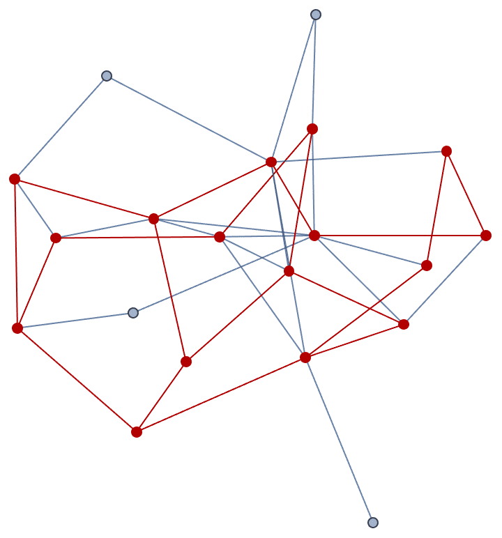
Display the Kuratowski subgraph on its own.
Graph[kur]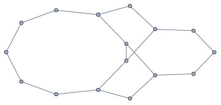
By smoothening the Kuratowski subgraph, we obtain either \(K_5\) or \(K_{3,3}\).
IGSmoothen@Graph[kur]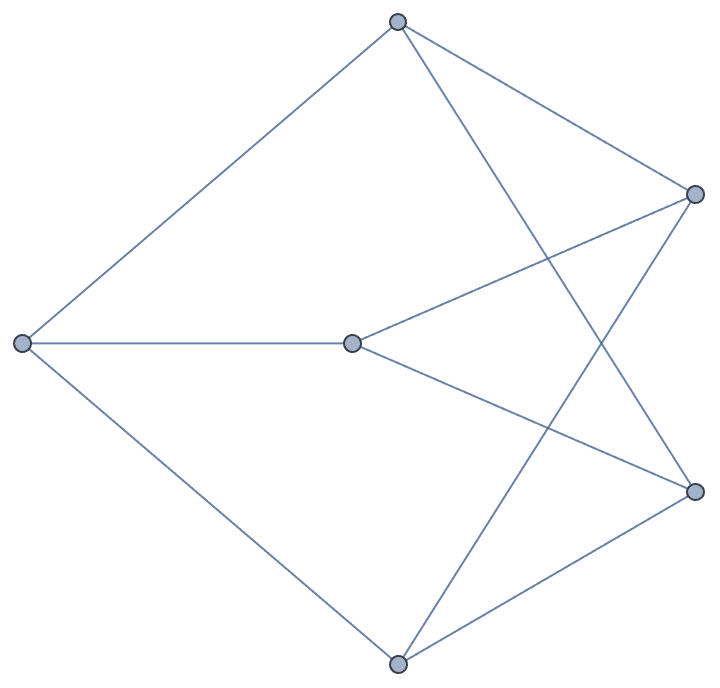
IGHomeomorphicQ[Graph[kur], #] & /@ {CompleteGraph[5],
CompleteGraph[{3, 3}]}{False, True}
For planar graphs, {} is returned.
IGKuratowskiEdges@CycleGraph[5]{}
?IGFaces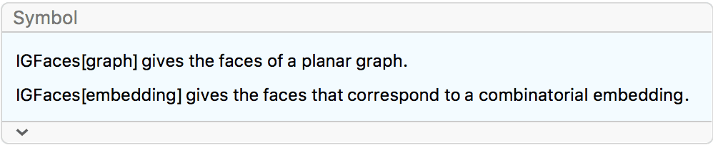
IGFaces returns the faces of a planar graph, or the
faces corresponding to a specific (not necessarily planar) embedding.
The faces are represented by a counter-clockwise ordering of vertices.
The current implementation ignores self-loops and multi-edges.
The faces of a planar graph are unique if the graph is
3-vertex-connected. This can be checked using
KVertexConnectedGraphQ.
g = GraphData["DodecahedralGraph"]
IGFaces[g]{{1, 14, 9, 10, 15}, {1, 15, 4, 8, 16}, {1, 16, 7, 3, 14}, {2, 5, 11, 12, 6}, {2, 6, 20, 18, 13}, {2, 13, 17, 19, 5}, {3, 7, 11, 5, 19}, {3, 19, 17, 9, 14}, {4, 15, 10, 18, 20}, {4, 20, 6, 12, 8}, {7, 16, 8, 12, 11}, {9, 17, 13, 18, 10}}
KVertexConnectedGraphQ[g, 3]True
If the graph is not connected and has \(C\) connected components, then \(C-1\) faces will be redundant.
g = IGDisjointUnion[{CycleGraph[3], CycleGraph[3]},
VertexLabels -> Automatic]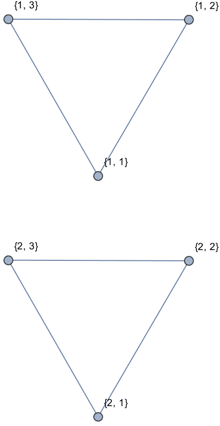
IGFaces[g]{{{1, 1}, {1, 2}, {1, 3}}, {{1, 1}, {1, 3}, {1, 2}}, {{2, 1}, {2, 2}, {2, 3}}, {{2, 1}, {2, 3}, {2, 2}}}
In the above-drawn arrangement, the outer faces of the two triangles are the same face. However, one triangle could have been drawn inside of the other. Then the inner face of one would be the same as the outer face of the other. Thus the choice of faces to be eliminated as redundant is arbitrary, and is left up to the user.
IGFaces can also be used with a non-planar combinatorial
embedding. The below embeddings both belong to the 4-vertex complete
graph, however, only the first is planar.
emb1 = <|1 -> {2, 3, 4}, 2 -> {1, 4, 3}, 3 -> {2, 4, 1},
4 -> {3, 2, 1}|>;
emb2 = <|1 -> {2, 4, 3}, 2 -> {4, 3, 1}, 3 -> {1, 2, 4},
4 -> {3, 1, 2}|>;IGFaces[emb1]{{1, 2, 3}, {1, 3, 4}, {1, 4, 2}, {2, 4, 3}}
IGFaces[emb2]{{1, 2, 3, 1, 4, 3, 2, 4}, {1, 3, 4, 2}}
Determine the genus \(g\) of an embedding belonging to a connected graph based on its face count \(F\), vertex count \(V\), and edge count \(E\), using the formula for the Euler characteristic \(2g-2=\chi =V-E+F\).
genus[emb_?
IGEmbeddingQ] := (2 + Total[Length /@ emb]/2 - Length[emb] -
Length@IGFaces[emb])/2genus /@ {emb1, emb2}{0, 1}
?IGDualGraph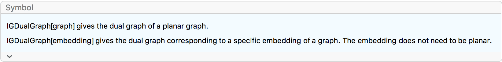
IGDualGraph returns a dual graph of a planar graph, or
the dual corresponding to a specific embedding. The ordering of the dual
graph’s vertices is consistent with the result of
IGFaces.
Limitations:
Multi-edges and self-loops are currently ignored.
The result is always a simple graph. No multi-edges or self-loops are generated
The dual of a simple 3-vertex-connected graph is simple and unique, thus such graphs are not affected by the above limitations.
TableForm[
Table[{CompleteGraph[k], IGDualGraph@CompleteGraph[k]}, {k, 1, 4}],
TableHeadings -> {None, {"graph", "dual"}}
]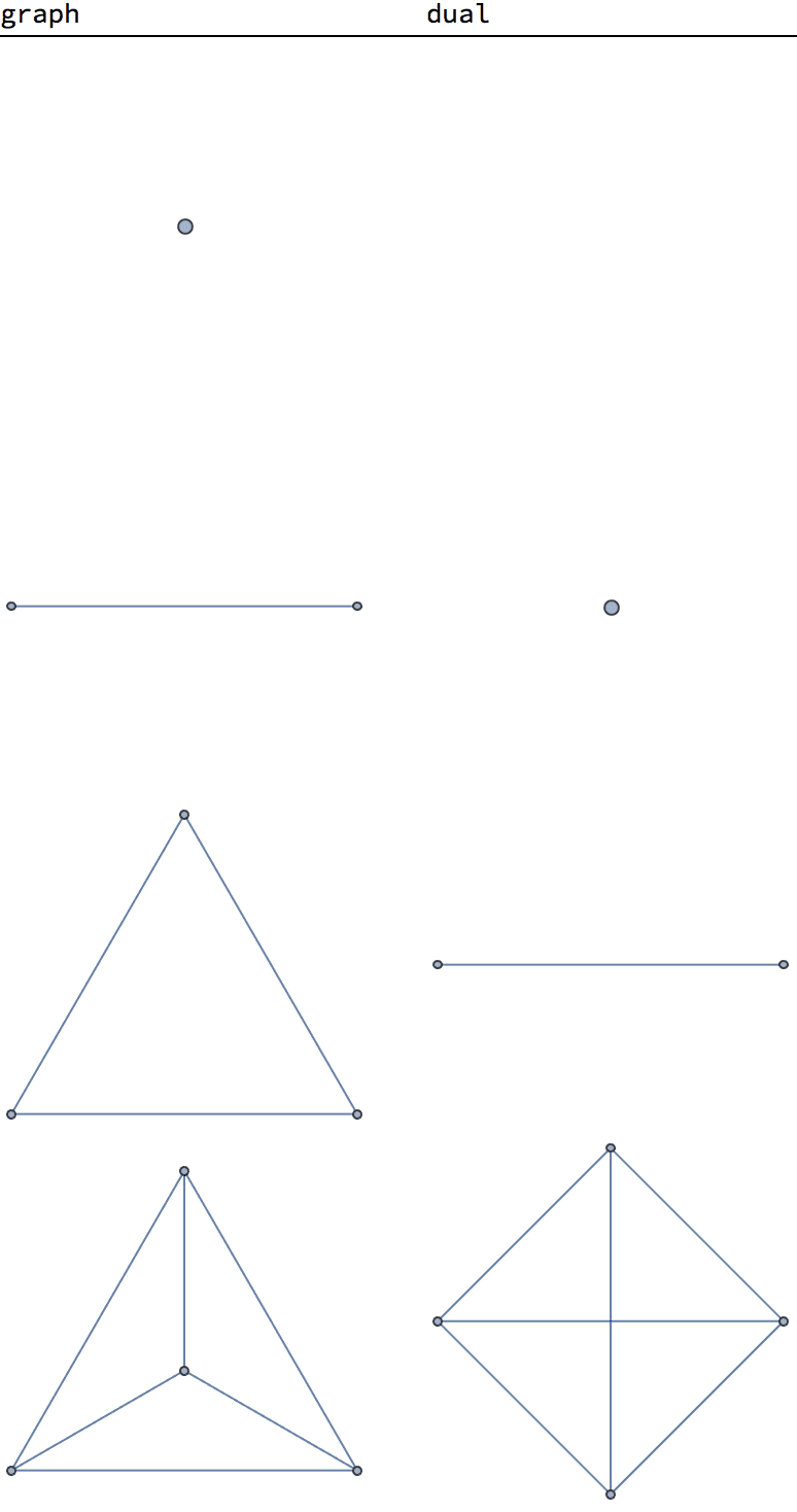
Currently, if the input is a graph, it must be planar.
IGDualGraph[CompleteGraph[5]]![]()
$Failed
If the input is a combinatorial embedding, it does not need to be planar.
emb = <|1 -> {2, 4, 3}, 2 -> {4, 3, 1}, 3 -> {1, 2, 4},
4 -> {3, 1, 2}|>;
IGPlanarQ[emb]False
IGDualGraph[emb]![]()
Find the dual of a square lattice graph. The dual graph also includes the outer face as a vertex.
IGSquareLattice[{5, 5}]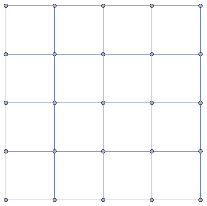
IGDualGraph[%]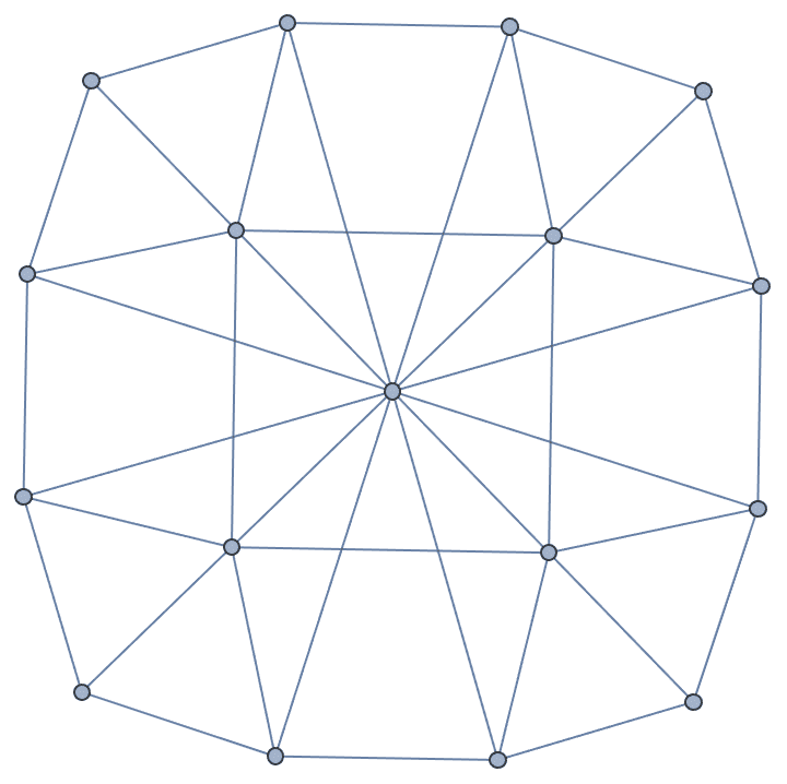
The dual is unique if the graph is 3-vertex-connected. This can be
verified using KVertexConnectedGraphQ. In this case,
IGDualGraph@IGDualGraph[g] is isomorphic to
g.
g = GraphData["IcosahedralGraph"]
dg = IGDualGraph[g]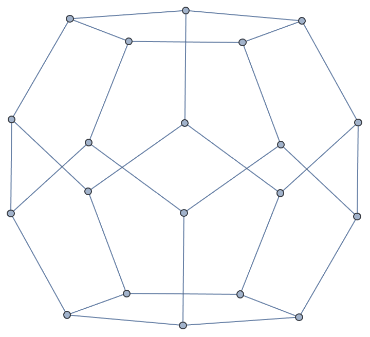
IGIsomorphicQ[dg, GraphData["DodecahedralGraph"]]True
IGIsomorphicQ[IGDualGraph[dg], g]True
If the graph is not connected, the dual of each component is effectively computed separately.
IGDualGraph@IGDisjointUnion[{CycleGraph[3], CycleGraph[3]}]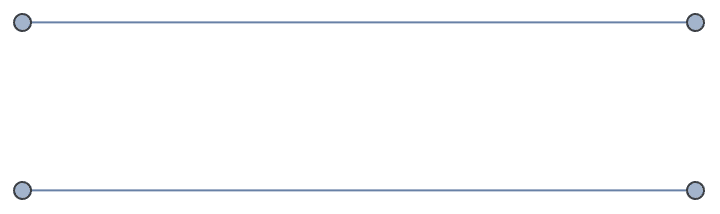
?IGEmbeddingQ
IGEmbeddingQ checks if an embedding is valid, and
whether it belongs to a graph without self-loops and multi-edges.
This is a valid combinatorial embedding of the graph
1 <-> 3 <-> 2.
IGEmbeddingQ[<|1 -> {3}, 2 -> {3}, 3 -> {1, 2}|>]True
The following embeddings do not belong to simple (i.e. loop free and multi-edge free) graphs:
IGEmbeddingQ[<|1 -> {3}, 2 -> {3, 3}, 3 -> {1, 2, 2}|>]False
IGEmbeddingQ[<|1 -> {1, 2}, 2 -> {1}|>]False
The following embedding is not valid because it does not contain the
arc 2 \[DirectedEdge] 1 but it does contain
1 \[DirectedEdge] 2.
IGEmbeddingQ[<|1 -> {2}, 2 -> {}|>]False
?IGPlanarEmbedding
IGPlanarEmbedding computes a combinatorial embedding of
a planar graph. The current implementation ignores self-loops and
multi-edges.
g = IGShorthand["a:b:c:d -- a:b:c:d"]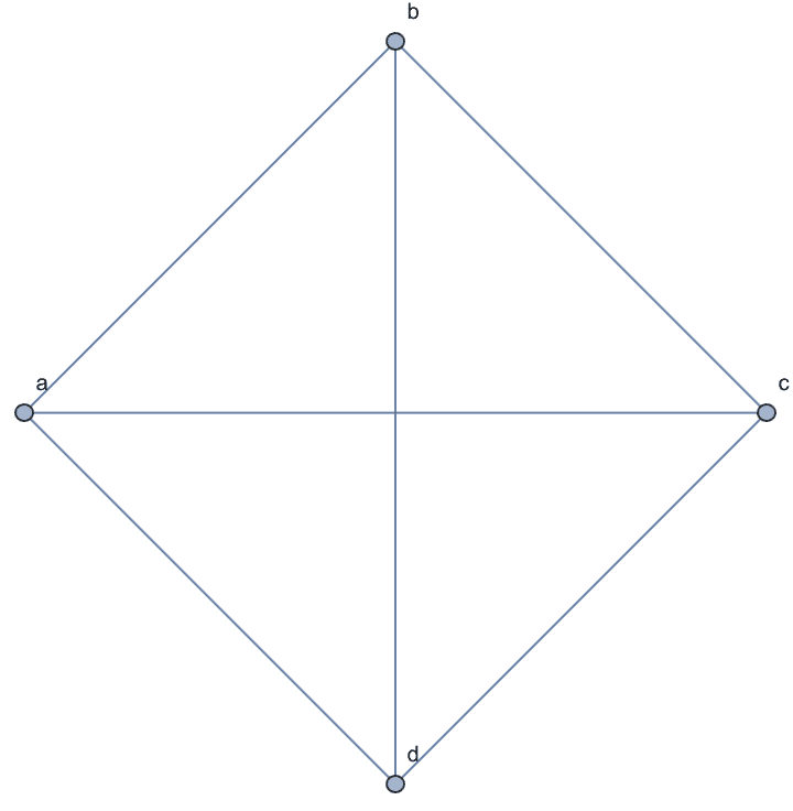
emb = IGPlanarEmbedding[g]<|"a" -> {"b", "c", "d"}, "b" -> {"a", "d", "c"}, "c" -> {"b", "d", "a"}, "d" -> {"c", "b", "a"}|>
The representation of a combinatorial embedding is also a valid
adjacency list, thus it can be easily converted back to an undirected
graph using IGAdjacencyGraph.
IGAdjacencyGraph[emb, VertexLabels -> Automatic]
?IGOuterplanarEmbedding
IGOuterplanarEmbedding returns an outerplanar
combinatorial embedding of a graph, if it exists. If the corresponding
graph is connected, then one face of such an embedding contains all
vertices of the graph.
g = IGTriangularLattice[{5, 2}]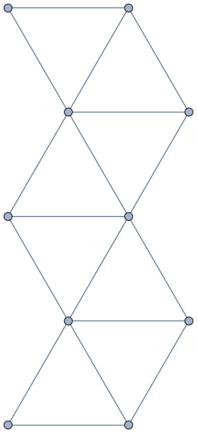
emb = IGOuterplanarEmbedding[g]<|1 -> {6, 2}, 2 -> {1, 6, 7, 8, 3}, 3 -> {2, 8, 4}, 4 -> {3, 8, 9, 10, 5}, 5 -> {4, 10}, 6 -> {2, 1, 7}, 7 -> {6, 8, 2}, 8 -> {7, 9, 4, 3, 2}, 9 -> {8, 10, 4}, 10 -> {9, 5, 4}|>
IGLayoutCircle@
IGReorderVertices[First@MaximalBy[Length]@IGFaces[emb], g]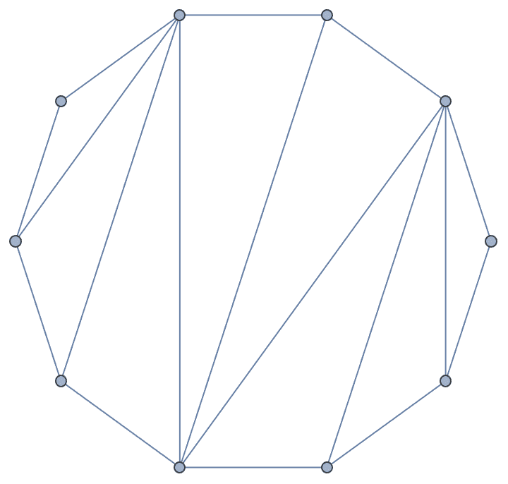
?IGCoordinatesToEmbedding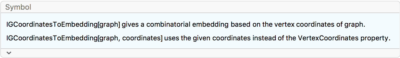
IGCoordinatesToEmbedding computes a combinatorial
embedding, i.e. a cyclic ordering of neighbours around each vertex,
based on the given vertex coordinates. By default, the coordinates are
taken from the VertexCoordinates property.
g = CompleteGraph[4, VertexLabels -> "Name"]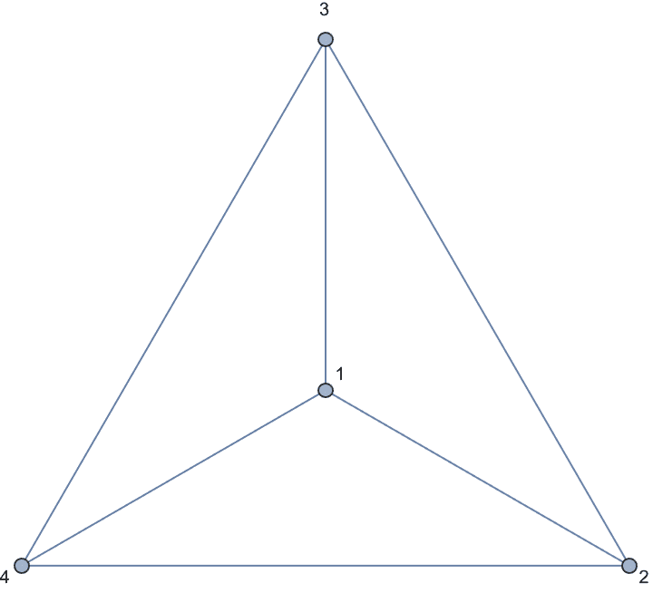
emb = IGCoordinatesToEmbedding[g]<|1 -> {4, 2, 3}, 2 -> {3, 1, 4}, 3 -> {4, 1, 2}, 4 -> {2, 1, 3}|>
The embedding can then be used to compute the faces of the graph …
IGFaces[emb]{{1, 4, 2}, {1, 2, 3}, {1, 3, 4}, {2, 4, 3}}
… or can be converted back to coordinates.
Graph[g, VertexCoordinates -> IGEmbeddingToCoordinates[emb]]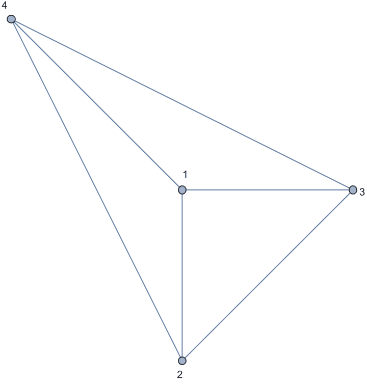
If we start with a non-planar graph layout, the embedding will not be planar either.
g = CompleteGraph[4, GraphLayout -> "SpringElectricalEmbedding",
VertexLabels -> "Name"]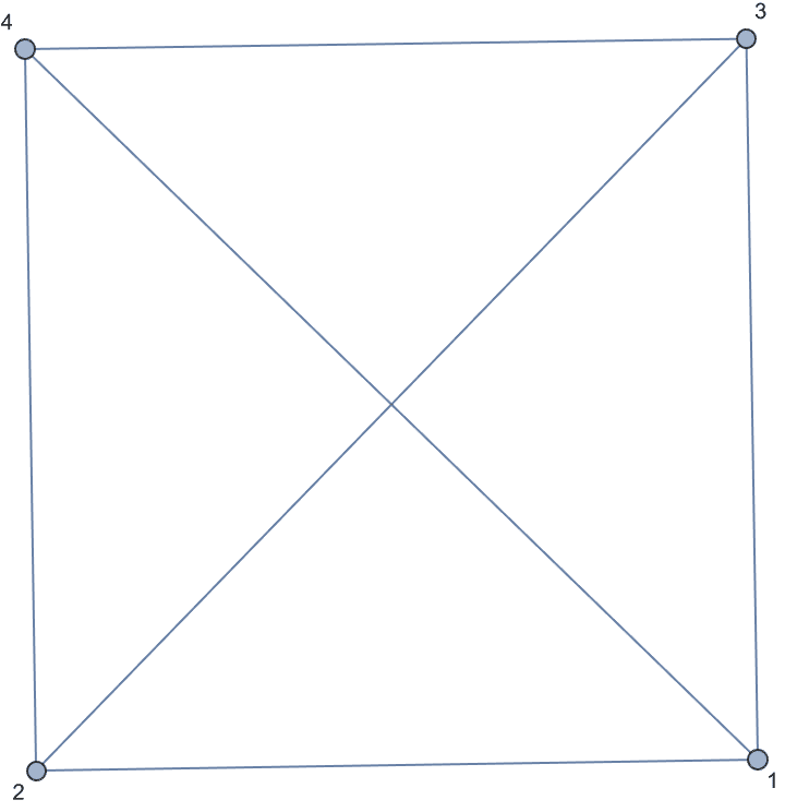
emb = IGCoordinatesToEmbedding[g]<|1 -> {2, 3, 4}, 2 -> {1, 3, 4}, 3 -> {4, 2, 1}, 4 -> {2, 1, 3}|>
IGFaces[emb]{{1, 2, 4, 3}, {1, 3, 2, 1, 4, 2, 3, 4}}
IGPlanarQ[emb]False
?IGEmbeddingToCoordinates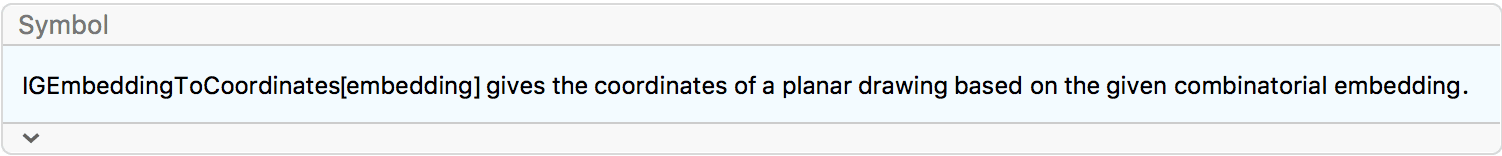
IGEmbeddingToCoordinates computes the coordinates of a
straight-line planar drawing based on the given combinatorial embedding,
using Schnyder’s algorithm.
emb1 = <|1 -> {2, 3, 4}, 2 -> {1, 4, 3}, 3 -> {2, 4, 1},
4 -> {3, 2, 1}|>;IGEmbeddingToCoordinates[emb1]{{1, 1}, {1, 0}, {2, 1}, {0, 2}}
The embedding must be planar.
emb2 = <|1 -> {2, 4, 3}, 2 -> {4, 3, 1}, 3 -> {1, 2, 4},
4 -> {3, 1, 2}|>;IGPlanarQ[emb2]False
IGEmbeddingToCoordinates[emb2]![]()
$Failed
?IGLayoutPlanar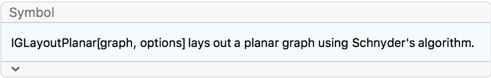
IGLayoutPlanar computes a layout of a planar graph
without edge crossings using Schnyder’s algorithm. The vertex
coordinates will lie on an \((n-2) \times
(n-2)\) integer grid, where \(n\) is the number of vertices.
Create a random planar graph and lay it out without edge crossings.
g = IGTryUntil[IGPlanarQ]@
RandomGraph[{10, 20}, VertexLabels -> "Name"]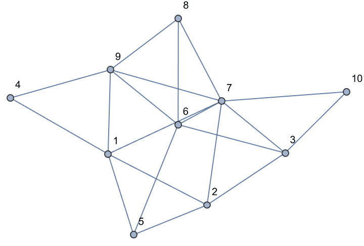
IGLayoutPlanar[g]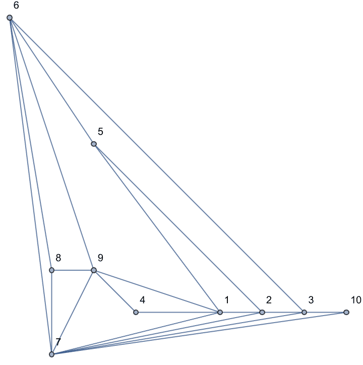
IGLayoutPlanar produces a drawing based on the
combinatorial embedding returned IGPlanarEmbedding. A
combinatorial embedding is a counter-clockwise ordering of the incident
edges around each vertex.
emb = IGPlanarEmbedding[g]<|1 -> {2, 5, 9, 4, 7}, 2 -> {1, 7, 3, 5}, 3 -> {2, 7, 10, 6}, 4 -> {1, 9}, 5 -> {2, 6, 1}, 6 -> {5, 3, 7, 8, 9}, 7 -> {6, 10, 3, 2, 1, 9, 8}, 8 -> {7, 9, 6}, 9 -> {8, 7, 4, 1, 6}, 10 -> {7, 3}|>
The embedding can also be used to directly compute coordinates for a drawing.
IGEmbeddingToCoordinates[emb]{{5, 1}, {6, 1}, {7, 1}, {3, 1}, {2, 5}, {0, 8}, {1, 0}, {1, 2}, {2, 2}, {8, 1}}
Graph[g, VertexCoordinates -> %]
?IGLayoutTutte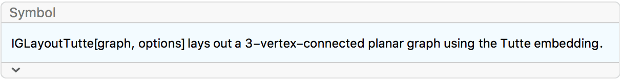
The Tutte embedding can be computed for a 3-vertex-connected planar graph. The faces of such a graph are uniquely defined. This embedding ensures that the coordinates of any vertex not on the outer face are the average of its neighbour’s coordinates, thus it is also called barycentric embedding.
IGLayoutTutte supports weighted graphs, and uses the
weights for computing barycentres.
The available options are:
"OuterFace" sets the planar graph face to use as the
outer face for the layout. The vertices of the face can be given in any
order. Use IGFaces to obtain a list of faces.By default, a largest face is chosen to be the outer one.
g = IGShorthand["1-2-3-1,4-5-6-4,1-4,2-5,3-6"]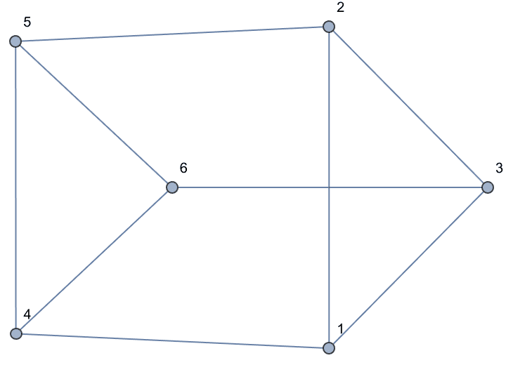
IGLayoutTutte[g]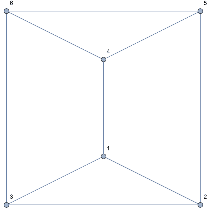
We can specify a different outer face manually.
IGLayoutTutte[g, "OuterFace" -> {5, 4, 6}]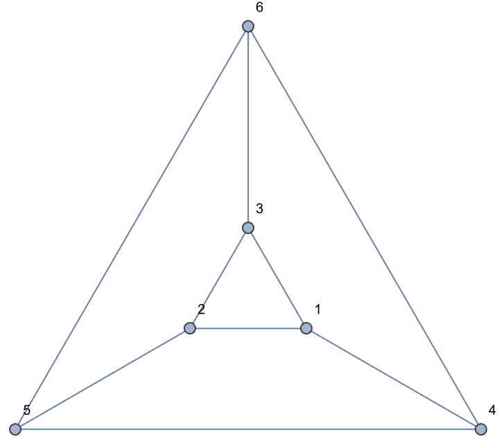
For some graphs, the best result is achieved when the outer face is not chosen to be a largest one.
g = GraphData["TutteGraph"];{IGLayoutTutte[g],
IGLayoutTutte[g, "OuterFace" -> {2, 8, 9, 10, 7, 6, 5, 4, 3}]}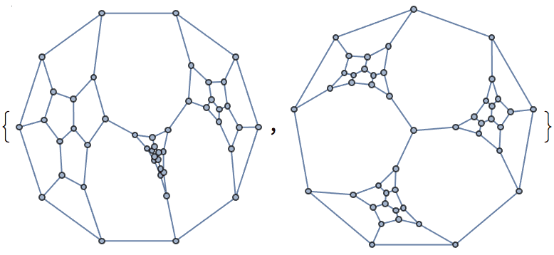
IGLayoutTutte requires a 3-vertex-connected planar
input.
IGLayoutTutte[CompleteGraph[5]]![]()
![]()
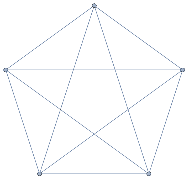
IGLayoutTutte[CycleGraph[5]]![]()
IGLayoutTutte will take into account edge weights. For a
weighted graph, the barycenter of neighbours is computed with a
weighting corresponding to the edge weights.
A disadvantage of the Tutte embedding is that the ratio of the shortest and longest edge it creates is often very large. This can be partially remedied by first computing an unweighted Tutte embedding, then setting edge weights based on the obtained edge lengths.
pg = IGLayoutTutte@GraphData["GreatRhombicosidodecahedralGraph"]
IGLayoutTutte@
IGEdgeMap[Apply[EuclideanDistance],
EdgeWeight -> IGEdgeVertexProp[VertexCoordinates], pg]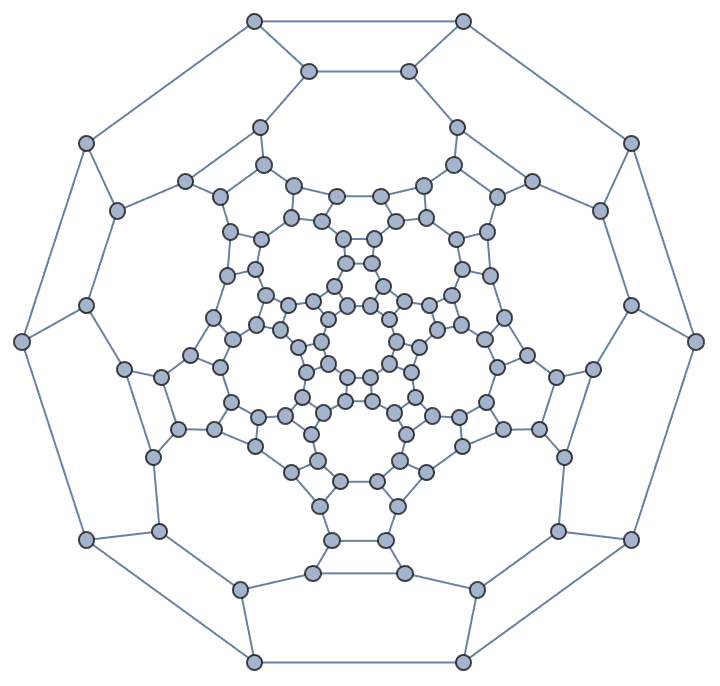
By applying a further power-transformation of the weight, we can fine-tune the layout.
Manipulate[
IGLayoutTutte[
IGEdgeMap[(EuclideanDistance @@ #)^power &,
EdgeWeight -> IGEdgeVertexProp[VertexCoordinates], pg],
VertexSize -> 1/2
],
{{power, 1}, 0.5, 3},
Initialization :> Needs["IGraphM`"]
]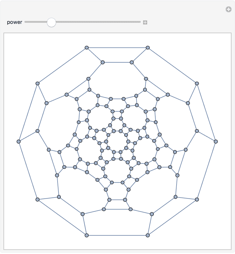
?IGMeshGraph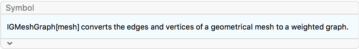
The available options are:
EdgeWeight sets either the explicit edge weights, or
the mesh property to be used as edge weights. The default value is
MeshCellMeasure. Use None to obtain an
unweighted graph.The following example demonstrates finding a shortest path on a geometric mesh.
mesh = DiscretizeRegion[
RegionDifference[Rectangle[{0, 0}, {3, 3}],
Rectangle[{0, 1}, {2, 2}]], MaxCellMeasure -> 0.02]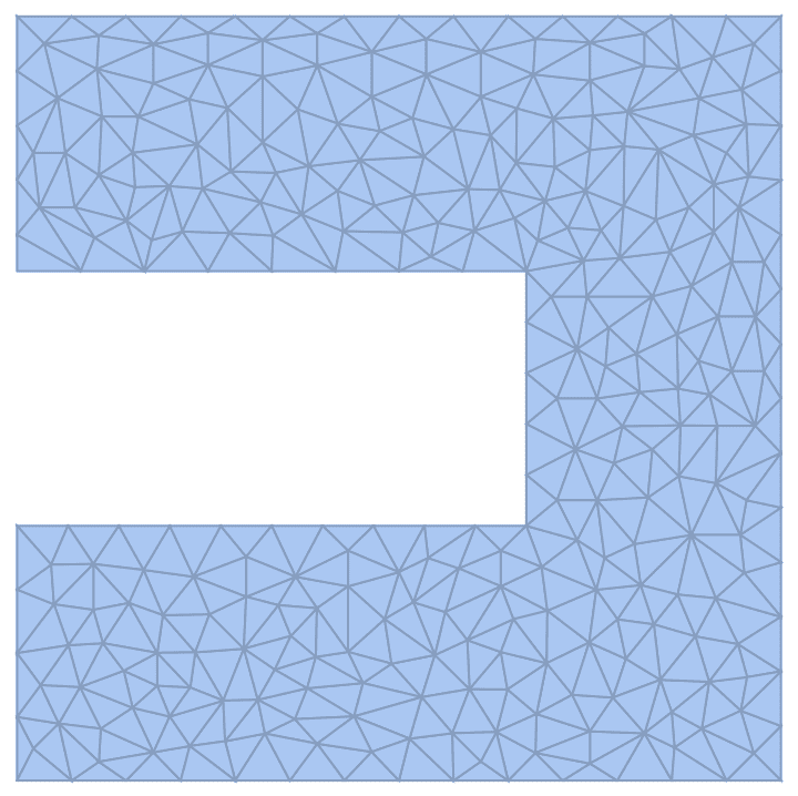
IGMeshGraph preserves the vertex coordinates, and uses
edge lengths as edge weights by default.
g = IGMeshGraph[mesh]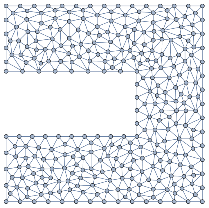
Find the corners.
st = First /@ Through[
{MinimalBy, MaximalBy}[VertexList[g],
Norm@PropertyValue[{g, #}, VertexCoordinates] &]
]{48, 20}
Highlight the shortest path.
HighlightGraph[g,
PathGraph@FindShortestPath[g, First[st], Last[st]],
Frame -> True, FrameTicks -> True
]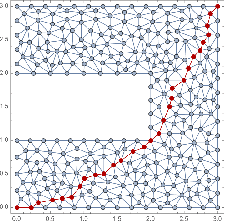
Find a Hamiltonian path on a mesh.
g = IGMeshGraph@DiscretizeRegion[Disk[], MaxCellMeasure -> 1/40];
HighlightGraph[g, PathGraph@FindHamiltonianPath[g],
GraphHighlightStyle -> "DehighlightHide"]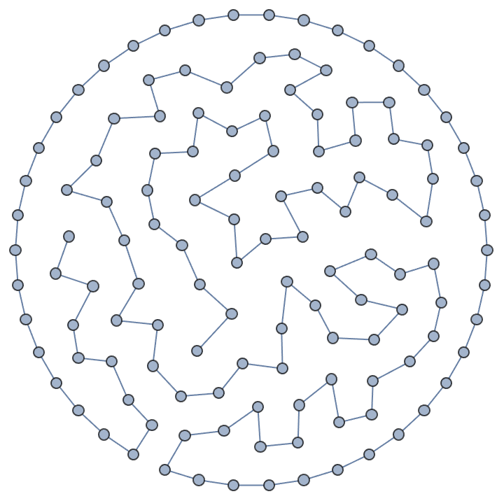
Get a spikey as a graph.
IGMeshGraph@PolyhedronData["Spikey", "BoundaryMeshRegion"]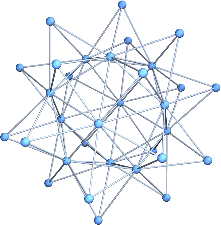
?IGMeshCellAdjacencyGraph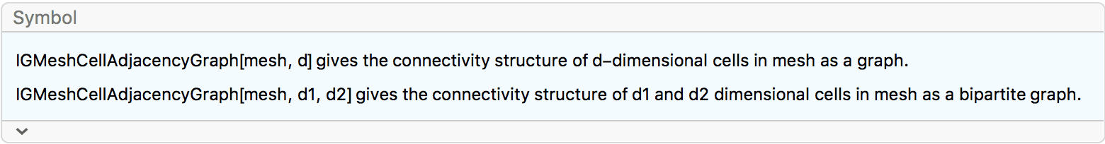
?IGMeshCellAdjacencyMatrix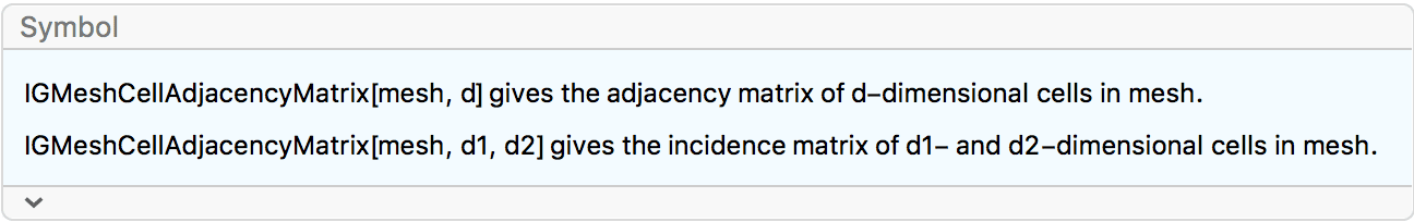
The available options for IGMeshCellAdjacencyGraph
are:
VertexCoordinates -> Automatic will use the mesh
cell centroids as vertex coordinates if the mesh is 2 or 3-dimensional.
The default is VertexCoordinates -> None, which does not
compute any coordinates.Compute the connectivity of mesh vertices (zero-dimensional cells).
mesh = DiscretizeRegion[Disk[], MaxCellMeasure -> 0.1]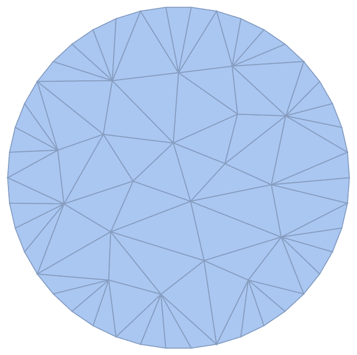
IGMeshCellAdjacencyGraph[mesh, 0, VertexCoordinates -> Automatic]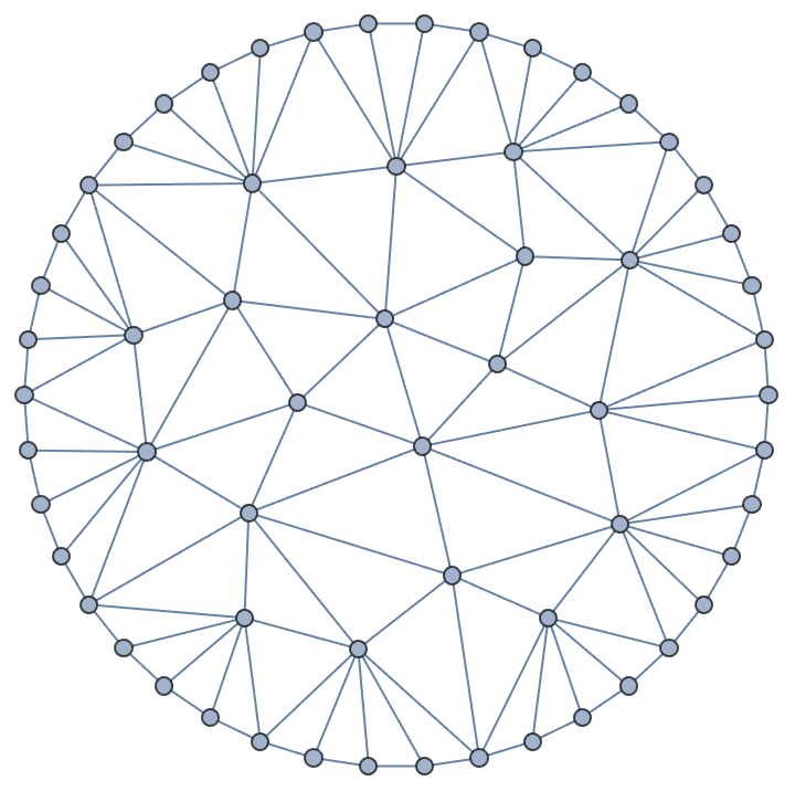
Compute the connectivity of faces (two-dimensional cells).
IGMeshCellAdjacencyGraph[mesh, 2]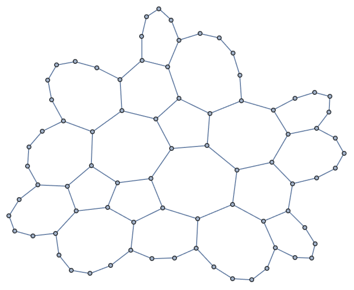
Create the graph of a Goldberg polyhedron.
IGMeshCellAdjacencyGraph[
BoundaryDiscretizeRegion[Ball[], PrecisionGoal -> 1,
MaxCellMeasure -> 0.5], 2,
VertexCoordinates -> Automatic]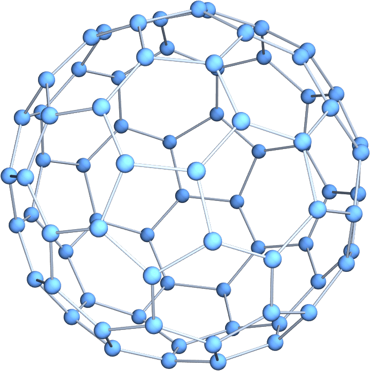
Compute the connectivity of faces and edges, and colour nodes based on whether they represent a face or an edge.
g = IGMeshCellAdjacencyGraph[
mesh, 2, 1,
VertexSize -> 0.9,
VertexStyle -> {EdgeForm[], {1, _} -> Red, {2, _} -> Black},
EdgeStyle -> Gray]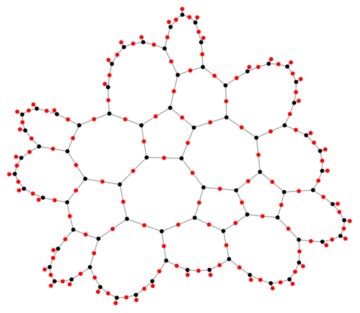
This is a bipartite graph.
IGBipartiteQ[g]True
The vertex names are the same as the mesh cell indices (see
MeshCellIndex).
VertexList[g] // Short![]()
Colour the faces of the mesh.
SetProperty[{mesh, {2, All}},
MeshCellStyle ->
ColorData[100] /@
IGVertexColoring@IGMeshCellAdjacencyGraph[mesh, 2]
]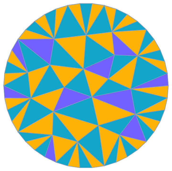
The edge-edge connectivity is identical to the line graph of the vertex-vertex connectivity.
IGIsomorphicQ[
LineGraph@IGMeshCellAdjacencyGraph[mesh, 0],
IGMeshCellAdjacencyGraph[mesh, 1]
]True
Compute the adjacency matrix of the vertex-vertex connectivity.
mesh = DiscretizeRegion[Sphere[],
PrecisionGoal -> 1.5, MaxCellMeasure -> 1, ImageSize -> Small]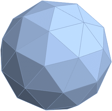
MatrixPlot@IGMeshCellAdjacencyMatrix[mesh, 0]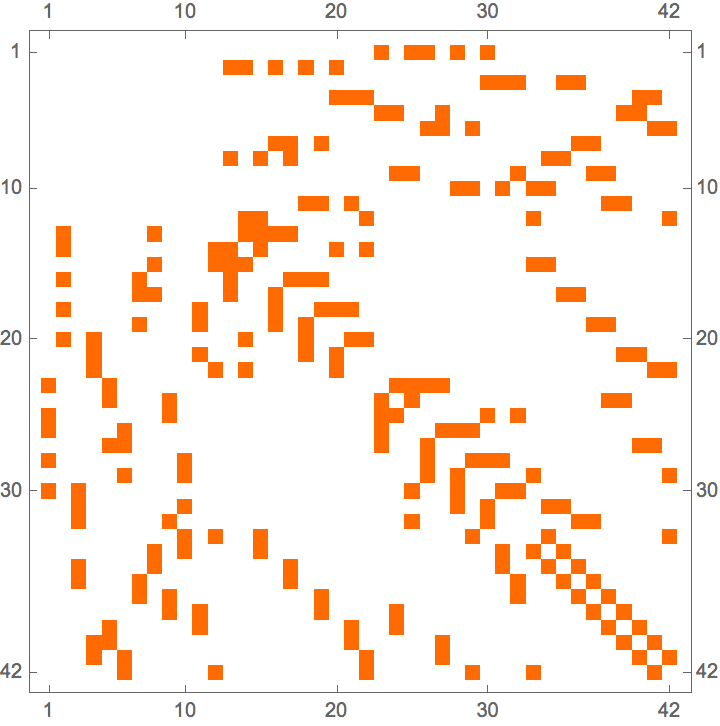
Compute the adjacency matrix of the edge-face connectivity.
bm = IGMeshCellAdjacencyMatrix[mesh, 1, 2]![]()
MatrixPlot[bm]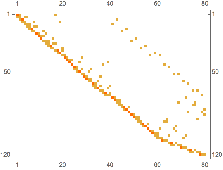
This is the (non-square) incidence matrix of a bipartite graph. The
graph can be reconstructed using
IGBipartiteIncidenceGraph.
Graph3D@IGBipartiteIncidenceGraph[bm]
Paint a Hamiltonian path on triangulation using a gradient of colours.
mesh = DiscretizeRegion[Disk[], MaxCellMeasure -> 1/50,
MeshCellStyle -> {1 -> None}];
path = FindHamiltonianPath@IGMeshCellAdjacencyGraph[mesh, 2];MeshRegion[
mesh,
MeshCellStyle ->
MapIndexed[#1 -> ColorData["Pastel"][First[#2]/Length[path]] &, path]
]
?IGLatticeMesh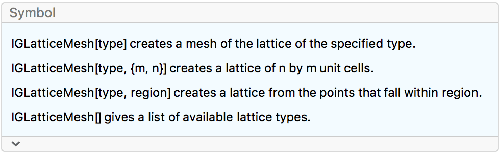
IGLatticeMesh can generate meshes of various periodic
tilings. IGMeshGraph and
IGMeshCellAdjacencyGraph can be used to convert these to
graphs. The primary use case is the easy generation of various lattice
graphs.
IGLatticeMesh[] returns the list of available lattices.
Let us explore them using a graphical interface.
Manipulate[IGLatticeMesh[type], {type, IGLatticeMesh[]},
Initialization :> Needs["IGraphM`"]]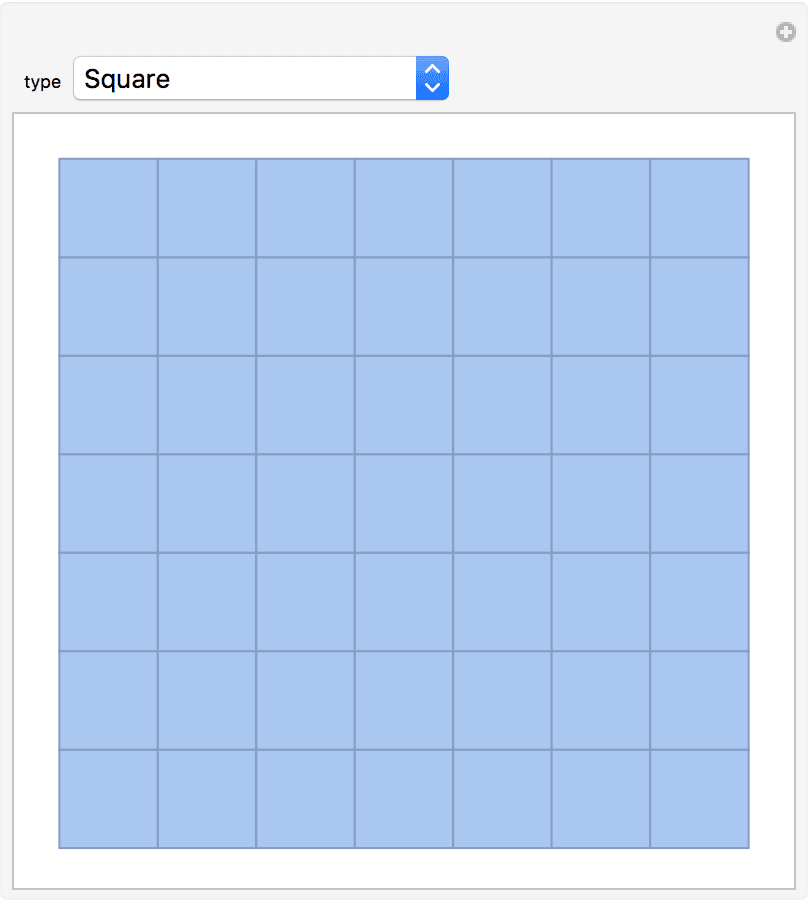
IGraph/M knows about a subset of the tilings available in
EntityClass["PeriodicTiling", All]. Use these entities to
obtain additional geometric information about the tilings.
Generate a kagome lattice consisting of 6 by 4 unit cells.
IGLatticeMesh["Trihexagonal", {6, 4}]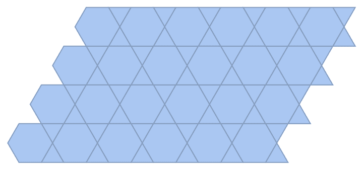
Create a hexagonal graph of 4 by 3 cells. Notice that the nodes are labelled with consecutive integers along the translation vectors of the lattice.
IGMeshGraph[
IGLatticeMesh["Hexagonal", {4, 3}],
VertexShapeFunction -> "Name", PerformanceGoal -> "Quality"]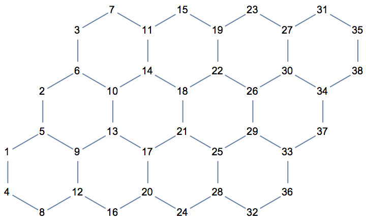
This specific node labelling allows for the creation of convenient directed lattices.
DirectedGraph[%, "Acyclic"]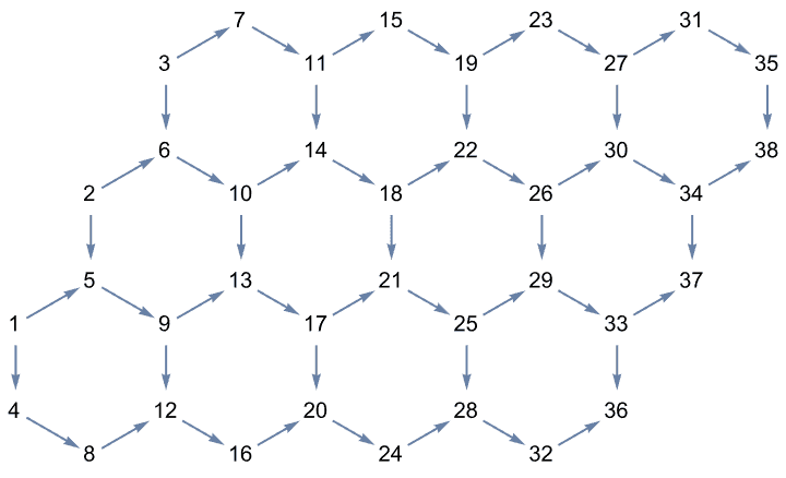
Create a hexagonal mesh from points that fall within a rectangular region.
IGLatticeMesh["Hexagonal", Rectangle[{0, 0}, {5, 5}]]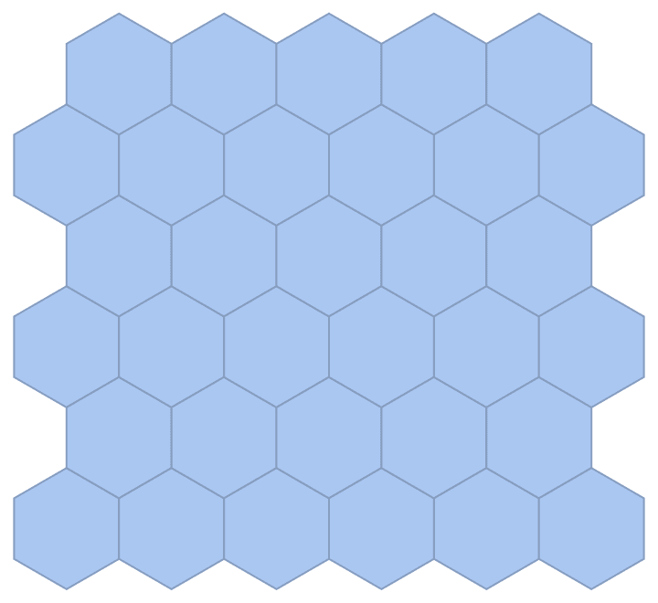
Create a hexagonal mesh from points that fall within a hexagonal region.
IGLatticeMesh["Hexagonal", Polygon@CirclePoints[3, 6]]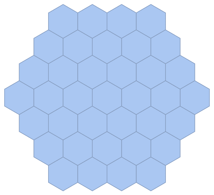
Create a triangular grid graph in the shape of a hexagon, as the face-adjacency graph of the above mesh.
IGMeshCellAdjacencyGraph[%, 2, VertexCoordinates -> Automatic]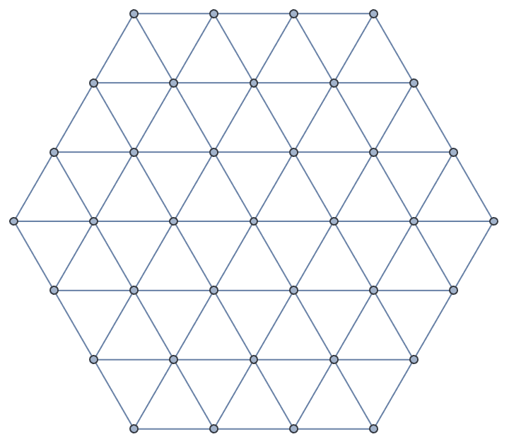
Create a face adjacency graph of the Cairo pentagonal tiling, and display it along with its mesh.
mesh = IGLatticeMesh["CairoPentagonal",
MeshCellStyle -> {1 -> Darker@Green, 2 -> LightGreen}];Show[
mesh,
IGMeshCellAdjacencyGraph[mesh, 2,
VertexCoordinates -> Automatic, GraphStyle -> "BasicBlack"],
ImageSize -> Medium
]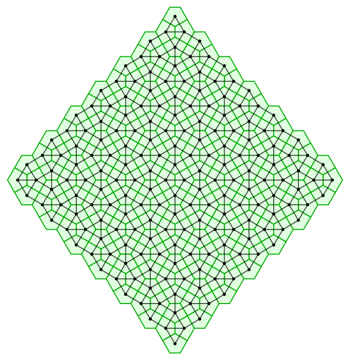
Compute a colouring of a periodic tiling so that neighbouring cells have different colours.
colorMesh[mesh_] :=
SetProperty[{MeshRegion[mesh, MeshCellStyle -> {1 -> White}], {2,
All}},
MeshCellStyle ->
ColorData[8] /@
IGMinimumVertexColoring@IGMeshCellAdjacencyGraph[mesh, 2]
]colorMesh@
IGLatticeMesh["Rhombille", Rectangle[{0, 0}, {10, 10}],
ImageSize -> Medium]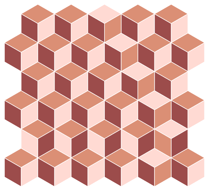
colorMesh@IGLatticeMesh["PentagonType2", {6, 4}, ImageSize -> Medium]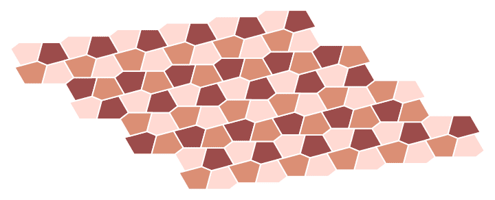
Explore the face-adjacency graphs of lattices. These correspond to the dual lattice.
Manipulate[
IGMeshCellAdjacencyGraph[IGLatticeMesh[type], 2,
VertexCoordinates -> Automatic],
{type, IGLatticeMesh[]}, Initialization :> Needs["IGraphM`"]
]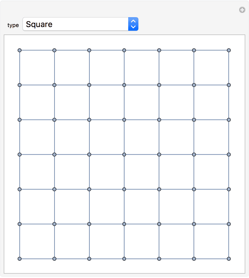
Make a maze through the faces of a lattice. We start by finding a spanning tree of the face-edge incidence graph of the lattice.
mesh = IGLatticeMesh["Square", Disk[{0, 0}, 9.5],
MeshCellStyle -> {1 | 2 -> GrayLevel[0.9]}];
t = IGRandomSpanningTree@IGMeshCellAdjacencyGraph[mesh, 2, 1];The walls of the maze will be the leaves of this tree which are edges.
walls = Cases[Pick[VertexList[t], VertexDegree[t], 1], {1, _}];We will remove two outer walls to serve as the
exits = SortBy[walls,
PropertyValue[{mesh, #}, MeshCellCentroid] . {1,
0.1} &][[{1, -1}]];Draw the maze.
MeshRegion[mesh,
MeshCellStyle ->
Thread[Complement[walls, exits] ->
Directive[AbsoluteThickness[4], Black]],
Epilog -> {Text["\!\(\*
StyleBox[\"\[LongRightArrow]\",\nFontWeight->\"Bold\",\n\
FontColor->RGBColor[1, 0, 0]]\)", #] & /@
PropertyValue[{mesh, exits}, MeshCellCentroid]}
]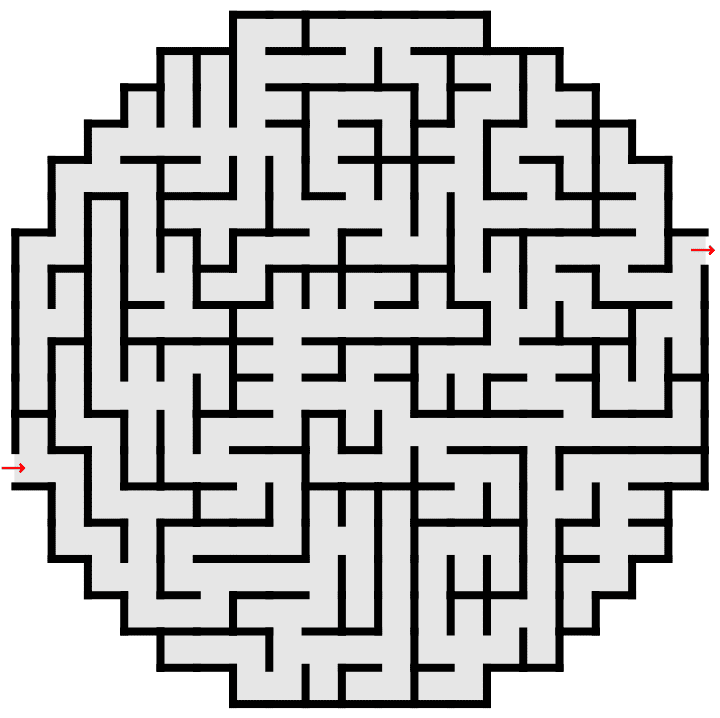
Create a Moiré pattern by superimposing two rotated hexagonal lattices.
m = IGLatticeMesh["Hexagonal", Polygon@CirclePoints[12., 6]];
Manipulate[
Show@Table[
MeshRegion[
TransformedRegion[m, RotationTransform[angle]],
MeshCellStyle -> {2 -> None, 1 -> AbsoluteThickness[1.5]},
PlotRange -> 13 {{-1, 1}, {-1, 1}}
],
{angle, {0, α}}
],
{{α, 0.15}, 0, 0.3},
Initialization :> Needs["IGraphM`"]
]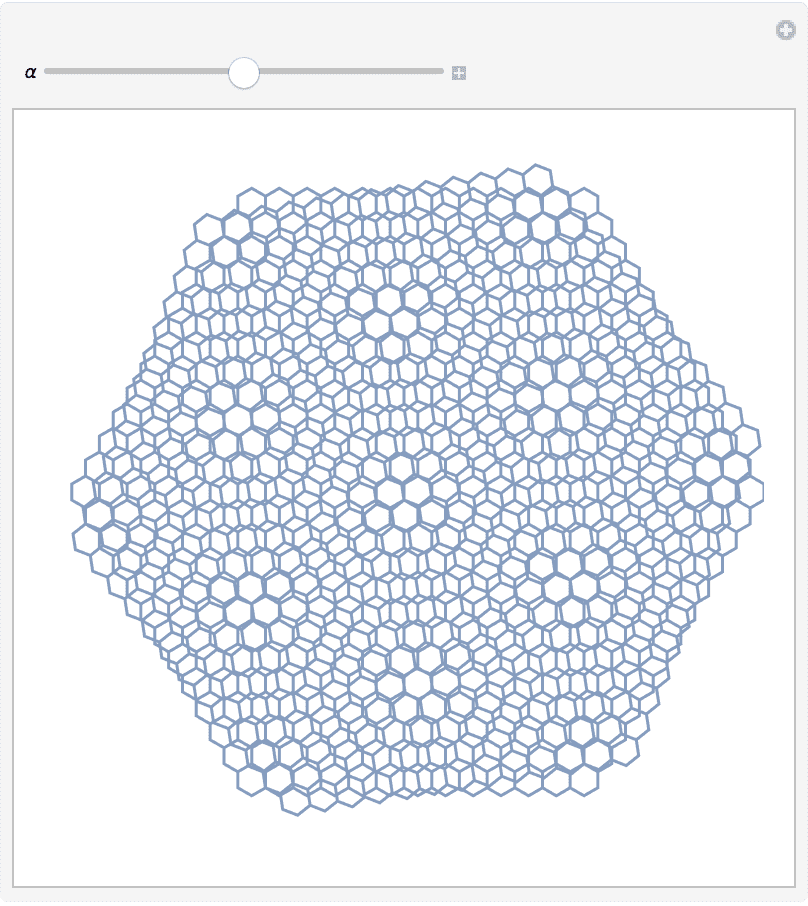
Proximity graphs are connectivity structures of geometric points based on geometric criteria. IGraph/M implements several proximity graphs for points in two-dimensional Euclidean space.
?IGDelaunayGraph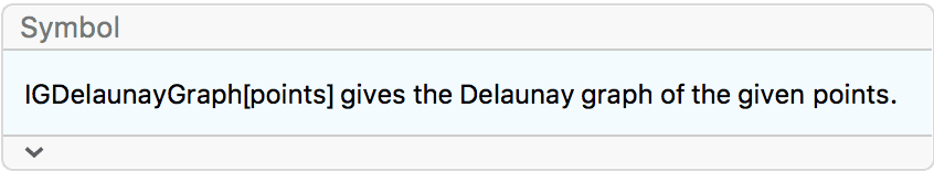
IGDelaunayGraph[points] creates computes the Delaunay
graph of the given points in one, two or three dimensions. It is
equivalent to IGMeshGraph@DelaunayMesh[points], but it is
faster and it supports collinear points in 2D and coplanar points in
3D.
IGDelaunayGraph works in 1D, 2D and 3D.
Table[
IGDelaunayGraph@RandomPoint[Ball@ConstantArray[0, dim], 30],
{dim, 1, 3}
]
IGDelaunayGraph works with collinear points in 2D …
IGDelaunayGraph[{{0, 0}, {2, 1}, {8, 4}, {6, 3}}]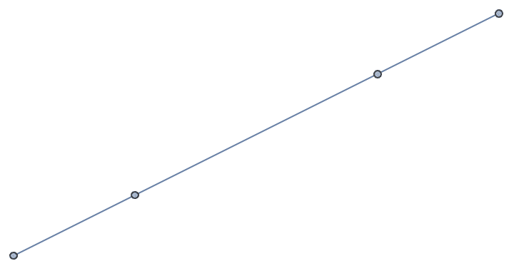
… or coplanar points in 3D.
IGDelaunayGraph[{{0, 0, 0}, {1, 0, 0}, {0, 1, 0}, {1, 1, 0}}]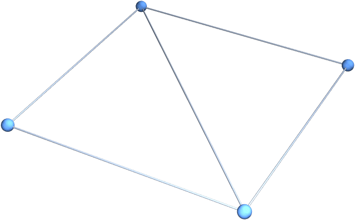
IGDelaunayGraph takes all the usual graph options.
IGDelaunayGraph[RandomReal[1, {10, 2}], GraphStyle -> "DiagramGold"]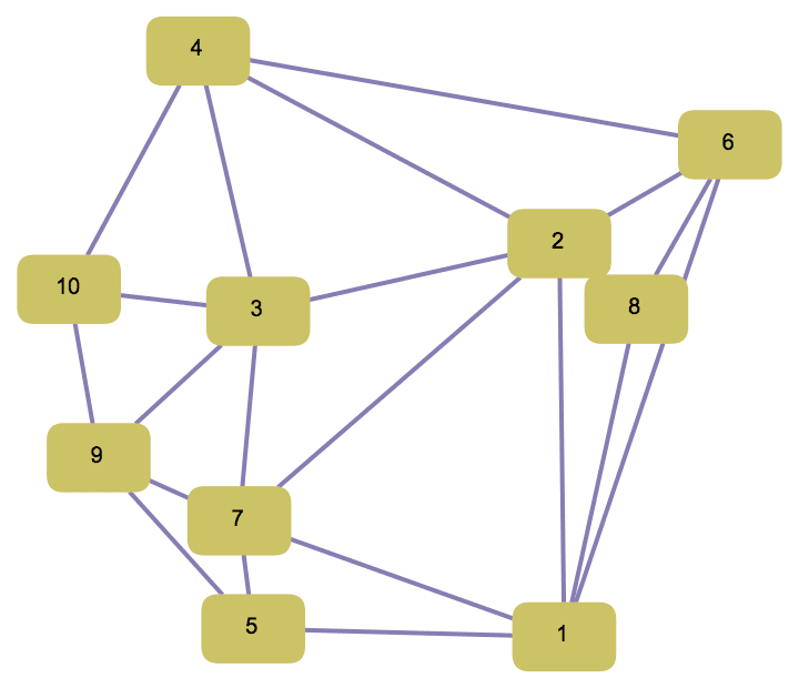
When there is more than one valid Delaunay triangulation, only one is returned.
IGDelaunayGraph@CirclePoints[5]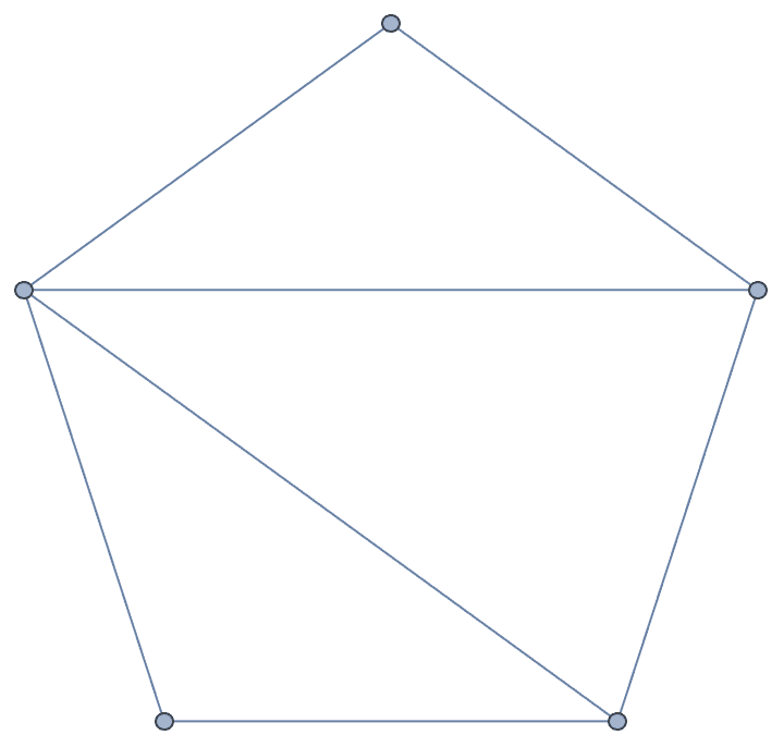
Find and plot an Euclidean minimum spanning tree of a set of points in three dimensions.
pts = RandomPoint[Ball[], 100];dg = IGDelaunayGraph[pts];
IGTakeSubgraph[dg,
IGSpanningTree@
IGEdgeMap[Apply[EuclideanDistance],
EdgeWeight -> IGEdgeVertexProp[VertexCoordinates], dg]
]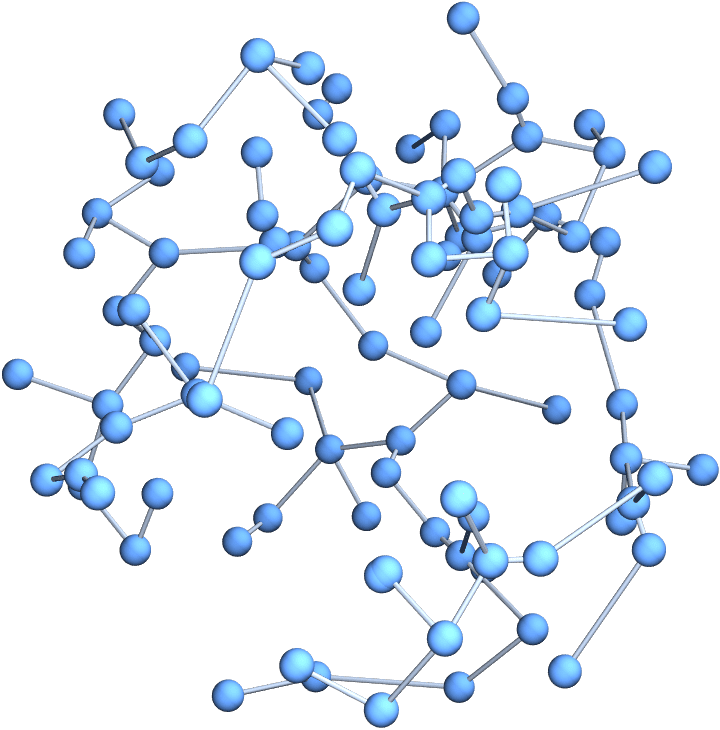
?IGLuneBetaSkeleton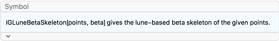
The lune-based β skeleton connects two points \(A\) and \(B\) when the intersection of two disks (a lune) having \(A\) and \(B\) on its boundary contains no other points.
For \(\beta \leq 1\), the lune is defined by disks of radius \(\text{\textit{AB}}/(2\beta )\).
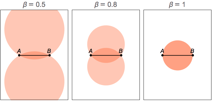
For \(\beta \geq 1\), the lune is defined by disks of radius \(\beta \text{\textit{AB}}/2\).
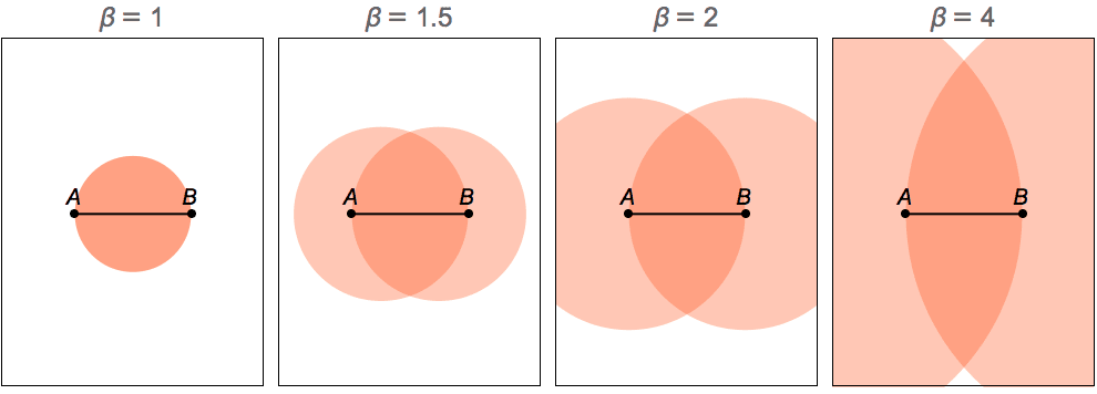
For \(\beta \geq 1\), the definition
generalizes to higher dimensions too. IGLuneBetaSkeleton
supports 2D and 3D point sets.
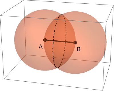
For \(\beta \geq 1\), the β skeleton is a subgraph of the Delaunay graph, thus its edges do not cross. For \(\beta <2\), it contains the Euclidean minimum spanning tree, thus it is connected. For \(\beta >2\), it is typically disconnected. For \(\beta =2\), it may be disconnected in special degenerate cases when three neighbouring points form an equilateral triangle.
The implementation of β skeleton computation is efficient only for \(\beta \geq 1\).
β skeletons can be used to reconstruct a shape from a set of points.
points = {{2.21, 3.83}, {2.5, 3.59}, {2.9, 3.49}, {3.33, 3.48}, {3.79,
3.55}, {4.27, 3.63}, {4.74, 3.65}, {5.25, 3.7}, {5.66,
3.65}, {5.98, 3.58}, {6.25, 3.47}, {6.43, 3.23}, {6.47,
2.86}, {6.35, 2.39}, {6.19, 2.02}, {5.98, 1.77}, {5.8,
1.57}, {5.51, 1.31}, {5.32, 0.94}, {5.19, 0.59}, {5.,
0.42}, {4.83, 0.31}, {4.62, 0.28}, {4.5, 0.37}, {4.54,
0.51}, {4.7, 0.58}, {4.82, 0.68}, {4.87, 0.91}, {4.87,
1.17}, {4.9, 1.6}, {4.91, 1.81}, {4.7, 1.7}, {4.47, 1.67}, {4.2,
1.7}, {3.89, 1.72}, {3.55, 1.84}, {3.53, 1.61}, {3.52,
1.33}, {3.51, 0.95}, {3.51, 0.48}, {3.4, 0.25}, {3.11,
0.21}, {3.02, 0.34}, {3.17, 0.5}, {3.16, 0.63}, {3.07, 0.94}, {3.,
1.27}, {2.93, 1.48}, {2.81, 1.61}, {2.6, 1.4}, {2.37,
1.29}, {2.11, 1.1}, {1.83, 0.99}, {1.66, 0.7}, {1.52,
0.46}, {1.33, 0.53}, {1.37, 0.76}, {1.47, 1.01}, {1.7,
1.3}, {1.91, 1.55}, {2.1, 1.73}, {2.29, 1.92}, {2.54,
1.78}, {1.97, 2.17}, {1.76, 2.5}, {1.6, 2.74}, {1.36,
2.98}, {1.29, 2.92}, {1.11, 2.88}, {0.87, 2.97}, {0.95,
3.16}, {0.95, 3.45}, {1.09, 3.78}, {1.31, 3.92}, {1.46,
4.01}, {1.22, 4.11}, {1.09, 4.31}, {1.09, 4.39}, {1.3,
4.34}, {1.49, 4.23}, {1.56, 4.07}, {1.95, 4.01}, {0.98,
3.91}, {0.88, 4.07}, {0.86, 4.26}, {1.04, 4.17}, {5.99,
1.32}, {6.21, 1.08}, {6.52, 0.85}, {6.53, 0.61}, {6.53,
0.41}, {6.46, 0.26}, {6.63, 0.16}, {6.84, 0.25}, {6.88,
0.47}, {6.89, 0.81}, {6.86, 1.12}, {6.69, 1.35}, {6.56,
1.65}, {6.55, 1.94}, {6.6, 2.4}, {6.61, 3.39}, {6.77,
3.72}, {6.81, 4.18}, {6.76, 4.6}, {6.7, 5.07}, {6.74,
5.51}, {6.99, 5.63}, {7.3, 5.71}, {7.41, 5.92}, {7.17,
6.11}, {6.74, 6.11}, {6.34, 5.86}, {6.17, 5.46}, {6.08,
4.98}, {6.15, 4.57}, {6.25, 4.19}, {6.21, 3.77}};IGLuneBetaSkeleton[points, #, PlotLabel -> #] & /@ {0.8, 1, 2, 5}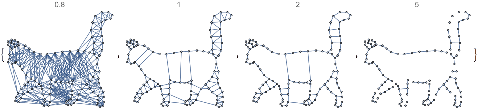
IGLuneBetaSkeleton works in 3D for \(\beta \geq 1\).
IGLuneBetaSkeleton[RandomPoint[Ball[], 20], 1.5]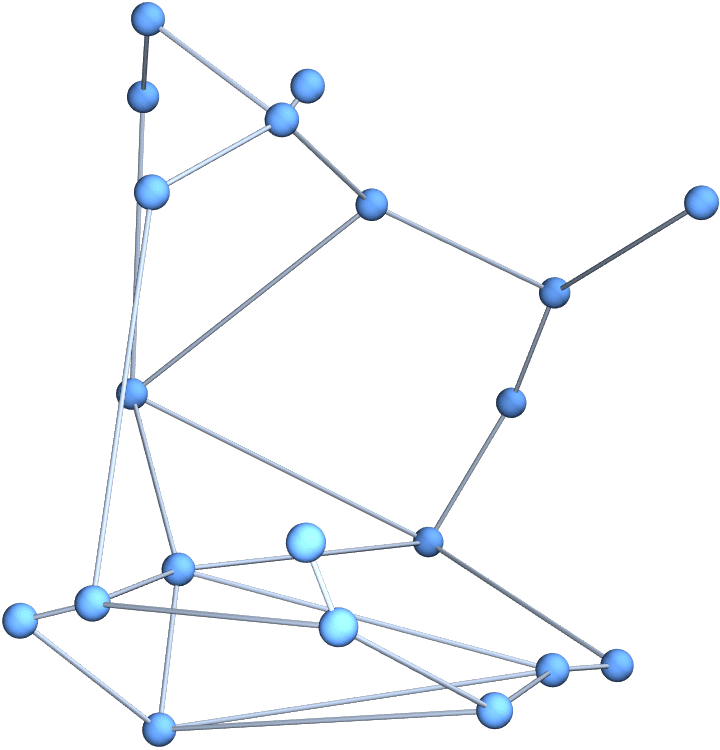
IGLuneBetaSkeleton[RandomPoint[Ball[], 20], 0.5]![]()
$Failed
Create a β-skeleton interactively. Point can be dragged around. To create or delete points, use -click on macOS, -click on Windows or --click on Linux.
DynamicModule[{pt = CirclePoints[0.5, 3], beta = 1.0},
Grid[List /@ {
Row[{Text@HoldForm[β], Spacer[10],
Slider[Dynamic[beta], {1/2, 4}], Spacer[10],
Text@Dynamic@NumberForm[beta, {3, 3}]}],
LocatorPane[
Dynamic[pt],
Dynamic@IGLuneBetaSkeleton[pt, beta,
PlotRange -> {{-1, 1}, {-1, 1}},
PlotRangePadding -> 0,
Frame -> True,
FrameTicks -> Automatic,
GridLines -> Automatic,
GraphStyle -> "BasicBlack",
ImageSize -> Medium, VertexShape -> None, VertexSize -> 0
],
LocatorAutoCreate -> True
]
}],
Initialization :> Needs["IGraphM`"]
]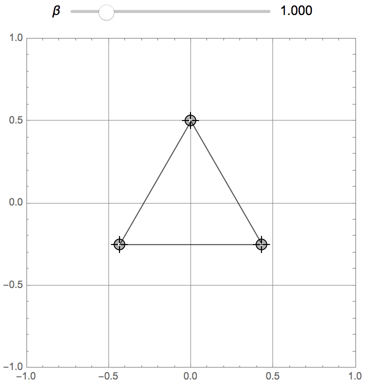
?IGCircleBetaSkeleton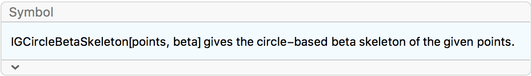
The circle-based β skeleton connects two points \(A\) and \(B\) if there is no other point \(C\) so that the angle \(\measuredangle A C B\) is less sharp the threshold
\[\theta =\left\{ \begin{array}{cc} \sin ^{-1}\left(\frac{1}{\beta }\right) & \beta \geq 1 \\ \pi -\sin ^{-1}(\beta ) & \beta \leq 1 \\ \end{array} \right.\]
This is equivalent to no point \(C\) being contained in the intersection or unions of the disks illustrated below.
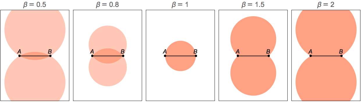
For \(\beta \leq 1\), the circle based and lune based beta skeletons coincide. For \(\beta >1\), the circle-based beta skeleton is a subgraph of the lune-based one.
Compute the circle-based β skeleton of a random point set.
IGCircleBetaSkeleton[
RandomVariate[NormalDistribution[0, 1], {100, 2}], 1.2]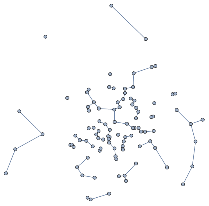
?IGRelativeNeighborhoodGraph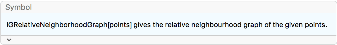
The relative neighbourhood graph is constructed from a set of points in space. Two points \(A\) and \(B\) are connected if and only if there is no other point \(C\) so that \(A C<A B\) and \(B C<A B\), with the inequialities being strict.
Most authors define the neighbourhood graph to coincide with a β-skeleton for \(\beta =2\). In IGraph/M, there is a subtle difference: the \(\beta =2\) skeleton connects points \(A\) and \(B\) when there is no point \(C\) so that \(A C\leq A B\) and \(B C\leq A B\). Therefore, three points forming an equilateral triangle are connected in the relative neighborhood graph, but disconnected in the \(\beta =2\) skeleton.
Compute the relative neighbourhood graph of a random set of points.
g = IGRelativeNeighborhoodGraph[RandomReal[1, {1000, 2}],
GraphStyle -> "VibrantColor", VertexSize -> {"Scaled", 0.005}]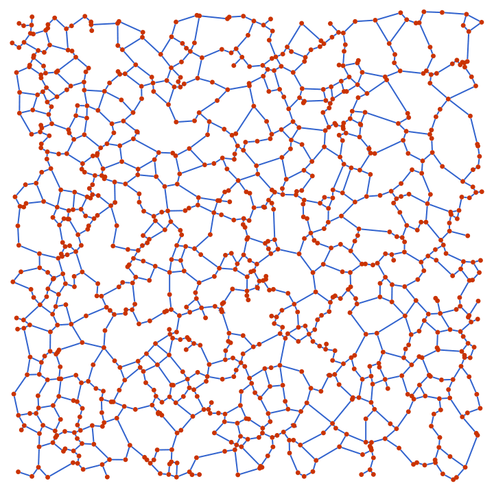
Assign edge lengths as weights …
g = IGDistanceWeighted[g];… and compute their distribution.
Histogram[IGEdgeProp[EdgeWeight][g]]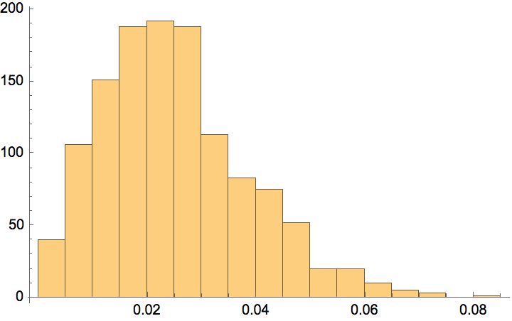
Plot the relative neighbourhood graph of African capitals.
capitals = CountryData["Africa", "CapitalCity"];
edges = IGIndexEdgeList@
IGRelativeNeighborhoodGraph@EntityValue[capitals, "Coordinates"];GeoGraphics[{{Red, Thick,
Line[capitals[[#]] & /@ edges]}, {PointSize[0.01],
Point[capitals]}}]
When the point set contain equilateral triangles, the relative neighbourhood graph may not coincide with the \(\beta =2\) skeleton.
pts = MeshCoordinates@IGLatticeMesh["Triangular"];{IGRelativeNeighborhoodGraph[pts], IGLuneBetaSkeleton[pts, 2]}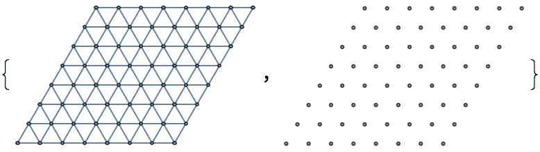
?IGGabrielGraph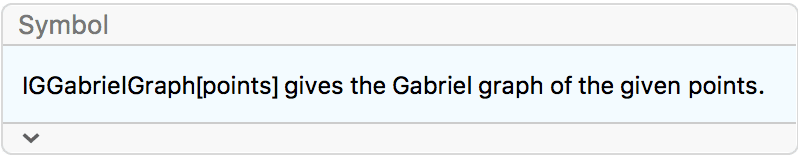
The Gabriel graph is constructed from a set of points in space. Two points \(A\) and \(B\) are connected if and only if no other point is contained in the disk of which \(A B\) is a diameter.
The Gabriel graph coincides with a β-skeleton for \(\beta =1\).
pts = RandomPoint[Disk[], 100];
g = IGGabrielGraph[pts]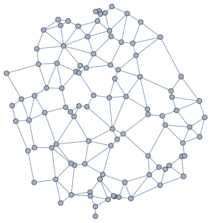
The Gabriel graph is a subgraph of the Delaunay graph.
HighlightGraph[IGMeshGraph@DelaunayMesh[pts], g]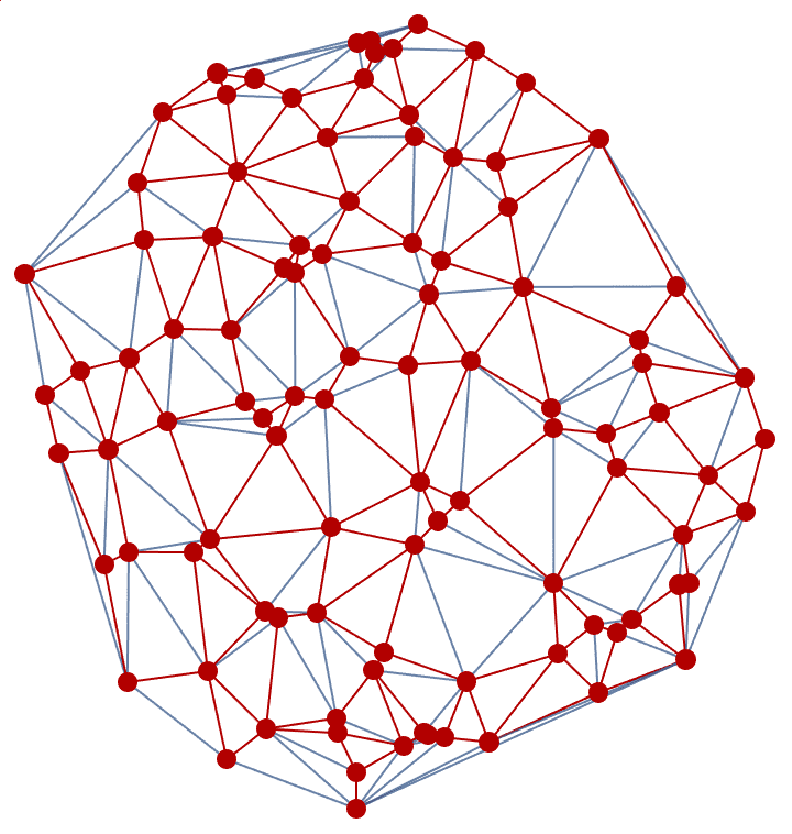
Convert the Gabriel graph to a MeshRegion object by finding its faces, and removing the outer face. Here we use the heuristic that for a graph generated from a random point set, the face with the most vertices is likely to be the outer face.
faces = IGFaces@IGCoordinatesToEmbedding[g];
faces = Delete[faces, Ordering[Length /@ faces, -1]];MeshRegion[pts, Polygon[faces]]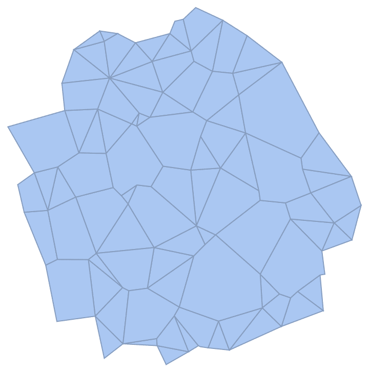
Compute a Gabriel graph in 3D.
IGGabrielGraph@
RandomVariate[MultinormalDistribution@IdentityMatrix[3], 100]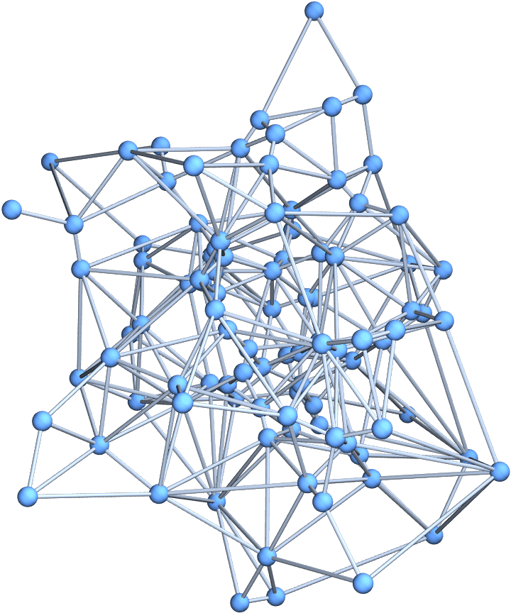
?IGBetaWeightedGabrielGraph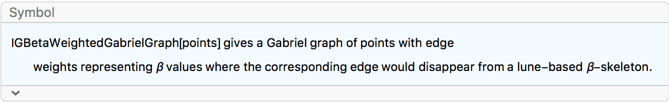
Experimental: This is experimental functionality that may change in the future.
IGBetaWeightedGabrielGraph[points] produces a Gabriel
graph in which edge weights represent threshold β values for lune-based
β-skeletons. Each edge is present in β-skeletons having a β parameter
smaller than the threshold stored in its weight.
Available options:
"BetaCutoff" -> cutoff only computes threshold β
values up cutoff. Larger thresholds will be returned as
Infinity. This option is intended to increase performance:
the lower the cutoff, the faster the computation. The default value is
Infinity, i.e. no cutoff.Colour edges by their inverse threshold β values:
pts = RandomPoint[Disk[], 60];g = IGBetaWeightedGabrielGraph[pts, GraphStyle -> "ThickEdge"] //
IGEdgeMap[ColorData["Rainbow"][1/#] &,
EdgeStyle -> IGEdgeProp[EdgeWeight]]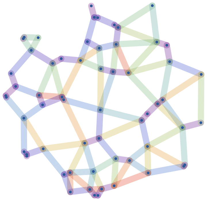
Plot the edge count of a lune-based β-skeleton of the same points as a function of β:
thresholds = IGEdgeProp[EdgeWeight][g];
ListLogLogPlot[
Transpose[{Reverse@Sort[thresholds], Range@Length[thresholds]}],
AxesLabel -> {"β", "edge count"}
]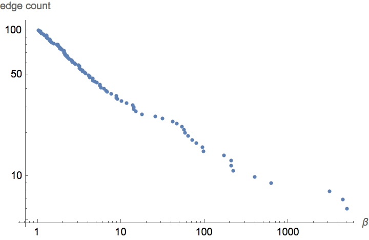
Show a percolation curve corresponding to edge removal in order of reverse threshold β:
ListPlot@
IGPercolationCurve@
Reverse@SortBy[EdgeList[g], PropertyValue[{g, #}, EdgeWeight] &]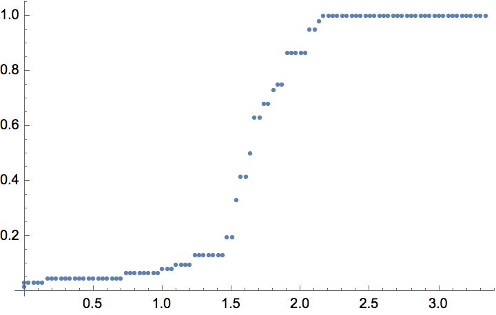
These functions perform basic operations on edge-weighted graphs without discarding edge weights. They are not based on the igraph C library.
IGWeightedAdjacencyGraph constructs an edge-weighted
graph from a weighted adjacency matrix. By default, 0
elements in the matrix are taken to indicate a lack of connection. An
alternative value may be specified to indicate the lack of
connections.
IGWeightedAdjacencyGraph takes the same options as
WeightedAjdacencyGraph.
?IGWeightedAdjacencyGraph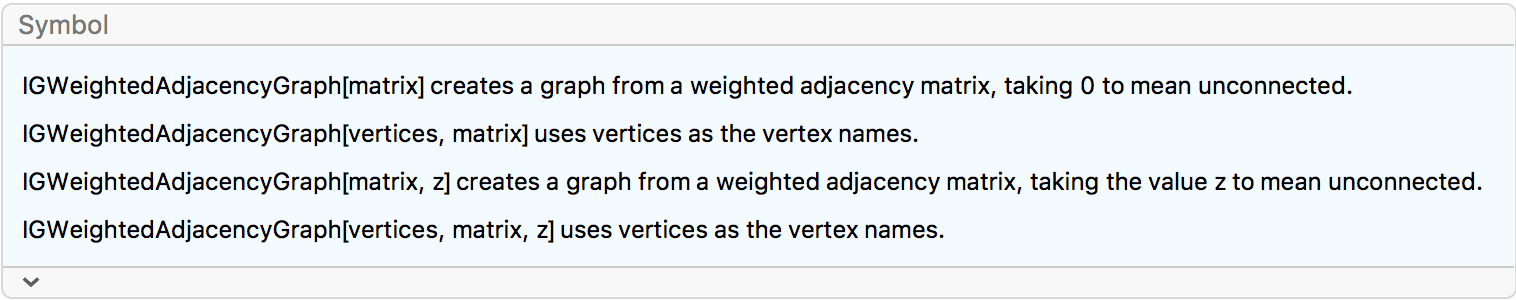
![]()
![]()
The built-in WeightedAdjacencyGraph uses
Infinity to indicate the lack of connection. This makes it
inconsistent with WeightedAdjacencyMatrix, which uses
0. The purpose of IGWeightedAdjacencyGraph is
to be able to easily interoperate with
WeightedAdjacencyMatrix, and to easily cycle a weighted
graph through an adjacency matrix representation.
wg = RandomGraph[{8, 15}, EdgeWeight -> {_ :> RandomReal[]}]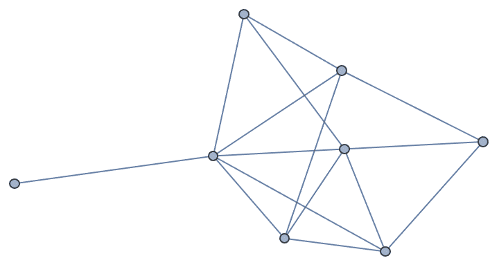
WeightedAdjacencyMatrix[wg] // MatrixForm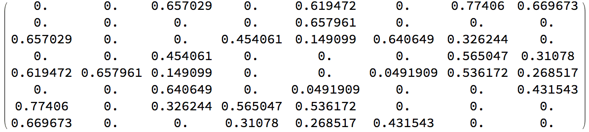
{IGWeightedAdjacencyGraph@WeightedAdjacencyMatrix[wg],
WeightedAdjacencyGraph@WeightedAdjacencyMatrix[wg]}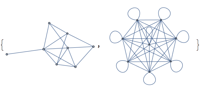
PropertyValue[%, EdgeWeight]$Failed
IGWeightedAdjacencyGraph[g, Infinity] is equivalent to
WeightedAdjacencyGraph[g].
![]()
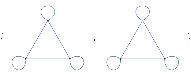
Use DirectedEdges -> True to force creating a
directed graph even from a symmetric matrix.
![]()
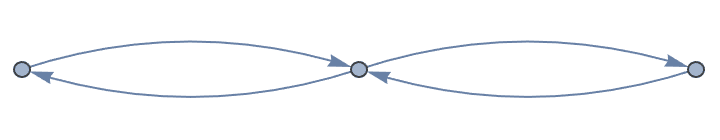
When the input matrix is not symmetric,
DirectedEdges -> False will cause the below-diagonal
part of the matrix to be ignored.
![]()
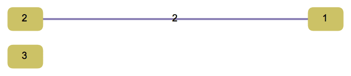
?IGWeightedAdjacencyMatrix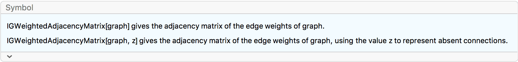
IGWeightedAdjacencyMatrix is equivalent to the built-in
WeightedAdjacencyMatrix with the difference that it allows
specifying the value to use for representing absent connections.
By default, absent connections are represented with 0.
This does not allow for distinguishing between absent connections and
connections with weight 0.
g = Graph[{1 <-> 2, 2 <-> 3},
EdgeWeight -> {2, 0}]![]()
IGWeightedAdjacencyMatrix[g] // MatrixForm![]()
IGWeightedAdjacencyMatrix[g, Infinity] // MatrixForm![]()
?IGEdgeWeightedQ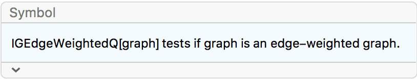
Unlike WeightedGraphQ, IGEdgeWeightedQ does
not return True for vertex-weighted graphs that have no
edge weights.
g = Graph[{1 <-> 2}, VertexWeight -> {1.2, 2.3}];IGEdgeWeightedQ[g]False
IGEdgeWeightedQ[SetProperty[g, EdgeWeight -> {1}]]True
?IGVertexWeightedQ
Unlike WeightedGraphQ, IGVertexWeightedQ
does not return True for edge-weighted graphs that have no
vertex weights.
g = Graph[{1 <-> 2}, EdgeWeight -> {3.1}];IGVertexWeightedQ[g]False
IGVertexWeightedQ[SetProperty[g, VertexWeight -> {2, 1}]]True
IGVertexStrength returns the strength of each vertex,
i.e. the total edge weight of edges adjacent to it.
?IGVertex*Strength
g = ExampleData[{"NetworkGraph", "EurovisionVotes"}];IGVertexStrength[g]{25, 12, 40, 17, 25, 21, 45, 60, 16, 50, 38, 6, 62, 51, 40, 38, 11, \ 63, 74, 15, 44, 29, 45, 48, 27, 29, 48, 24, 6, 18, 30, 63, 27, 27, \ 49, 83, 2, 43, 6, 28, 43, 57, 25, 91, 55, 40}
In- and out-strength can be calculated separately for directed graphs.
{IGVertexInStrength[g], IGVertexOutStrength[g]}{{11, 0, 30, 3, 19, 7, 20, 38, 4, 24, 13, 0, 40, 25, 20, 12, 5, 37, 52, 3, 22, 5, 21, 26, 7, 9, 22, 12, 0, 10, 7, 39, 5, 6, 27, 61, 0, 31, 0, 4, 17, 31, 5, 65, 39, 14}, {14, 12, 10, 14, 6, 14, 25, 22, 12, 26, 25, 6, 22, 26, 20, 26, 6, 26, 22, 12, 22, 24, 24, 22, 20, 20, 26, 12, 6, 8, 23, 24, 22, 21, 22, 22, 2, 12, 6, 24, 26, 26, 20, 26, 16, 26}}
IGVertexInStrength[g] + IGVertexOutStrength[g] == IGVertexStrength[g]True
Scale vertices by strength:
IGVertexMap[{"Scaled", 0.1 #} &,
VertexSize -> (Normalize[IGVertexStrength[#], Max] &), g]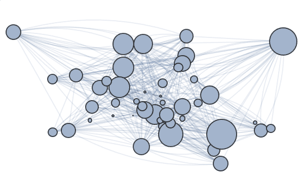
IGUnweighted[g] returns a version of the graph
g with edge weights removed.
?IGUnweighted
This function is useful for computing graph properties such as betweenness centrality without taking weights into account.
g = ExampleData[{"NetworkGraph", "EastAfricaEmbassyAttacks"}];IGBetweenness[g]{2., 2., 1., 0., 8., 0., 8.5, 23.5, 0.5, 14.5, 7., 3.5, 71.5, 3., 7., \ 0., 0., 30.}
IGBetweenness@IGUnweighted[g]{3.49167, 0.416667, 3.75, 0., 3.48333, 1.79167, 11.9167, 32.3417, \ 7.38333, 5.9, 6.65, 1.36667, 20.275, 8.45, 23.4833, 0., 0., 2.3}
IGDistanceWeighted[g] returns a weighted version of the
graph g, setting the weights of edges to the distance
between their endpoints. The distances are computed based on the
VertexCoordinates property.
?IGDistanceWeighted
The available options are:
DistanceFunction sets the function used to compute
distances. The default is EuclideanDistance.Create a Delaunay graph.
pts = RandomPoint[Disk[], 100];
g = IGDelaunayGraph[pts, GraphStyle -> "BasicBlack",
VertexSize -> {"Scaled", 0.03}]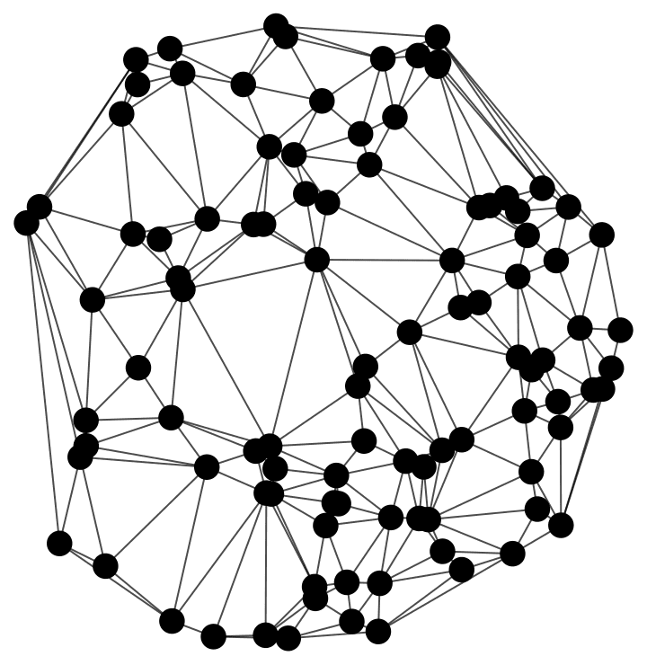
IGDelaunayGraph returns unweighted graphs.
IGEdgeWeightedQ[g]False
Set edge weights based on the geometrical distances between the edge endpoints.
wg = IGDistanceWeighted[g]
IGEdgeWeightedQ[wg]True
Edge weights are taken into account by many graph analysis functions.
IGVertexMap[ColorData["Rainbow"],
VertexStyle -> Rescale@*IGBetweenness] /@ {wg, g}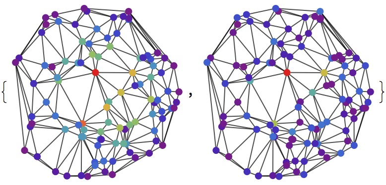
Compute the mean edge length.
Mean[IGEdgeProp[EdgeWeight][wg]]0.218076
Use Manhattan distances instead of Euclidean distances.
IGDistanceWeighted[g, DistanceFunction -> ManhattanDistance] //
IGEdgeProp[EdgeWeight] // Mean0.278232
IGDistanceWeighted[g] is effectively equivalent to the
following IGEdgeMap construct, but faster for several
specific distance functions:
wg1 = IGEdgeMap[Apply[EuclideanDistance],
EdgeWeight -> IGEdgeVertexProp[VertexCoordinates],
g]; // RepeatedTiming{0.000962632, Null}
wg2 = IGDistanceWeighted[g]; // RepeatedTiming{0.000309226, Null}
IGEdgeProp[EdgeWeight][wg1] == IGEdgeProp[EdgeWeight][wg2]True
?IGWeightedSimpleGraph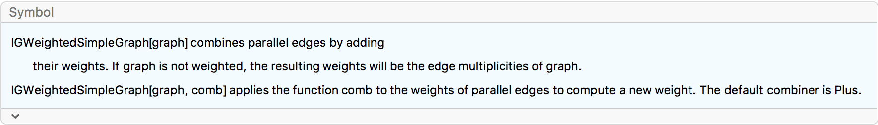
IGWeightedSimpleGraph creates an edge-weighted graph by
combining the weights of parallel edges. The default combiner function
is Plus. If the input is an unweighted graph, the resulting
weights will be the edge multiplicities of the input graph.
Available options:
SelfLoops -> False will discard self-loops. The
default is to keep them.Convert edge multiplicities to weights.
g = IGGrowingGame[30, 3]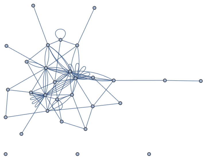
IGWeightedSimpleGraph[g] //
IGEdgeMap[AbsoluteThickness, EdgeStyle -> IGEdgeProp[EdgeWeight]]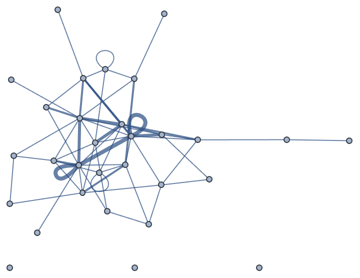
Discard self-loops and apply additional graph options.
IGWeightedSimpleGraph[g, SelfLoops -> False, PlotTheme -> "NeonColor"]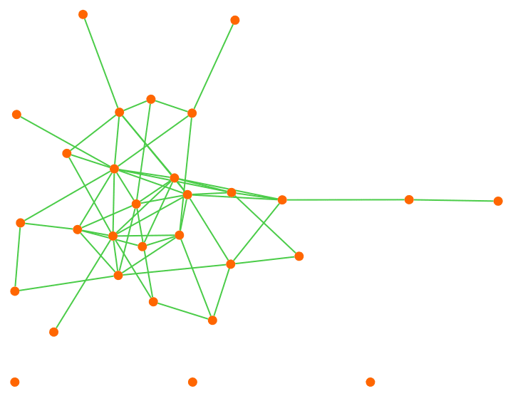
IGEdgeWeightedQ[%]True
Combine edge weights by adding, multiplying or averaging, as
controlled by the second argument of
IGWeightedSimpleGraph.
MatrixForm@WeightedAdjacencyMatrix@IGWeightedSimpleGraph[
Graph[{1 <-> 2, 1 <-> 2,
2 <-> 3}, EdgeWeight -> {2, 3, 4}],
#
] & /@ {Plus, Times, Mean[{##}] &}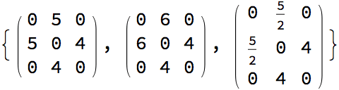
?IGWeightedUndirectedGraph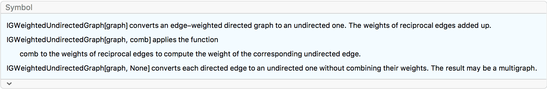
IGWeightedUndirectedGraph works like the built-in
UndirectedGraph, but preserves edge weights. The weights of
reciprocal edges will be combined with the given combiner function. By
default, Plus is used, i.e. they are added up.
IGWeightedUndirectedGraph[
Graph[{1 -> 2, 2 -> 1, 2 -> 3}, EdgeWeight -> {3, 4, 5}]
] // WeightedAdjacencyMatrix // MatrixForm![]()
Average weights instead of adding them.
IGWeightedUndirectedGraph[
Graph[{1 -> 2, 2 -> 1, 2 -> 3}, EdgeWeight -> {3, 4, 5}],
Mean[{##}] &
] // WeightedAdjacencyMatrix // MatrixForm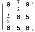
This function is not meant to be used with multigraphs. If the input is a multigraph, weights of parallel edges will be combined with the same combiner function that is used for reciprocal edges. This may lead to unexpected results, thus a warning is issued.
IGWeightedUndirectedGraph[
Graph[{1 -> 2, 1 -> 2, 2 -> 1, 2 -> 3}, EdgeWeight -> {3, 4, 4, 5}],
Mean[{##}] &
] // WeightedAdjacencyMatrix // MatrixForm![]()
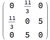
Use IGWeightedSimpleGraph to combine parallel edges
before converting the graph to undirected.
IGWeightedUndirectedGraph[
IGWeightedSimpleGraph[
Graph[{1 -> 2, 1 -> 2, 2 -> 1, 2 -> 3},
EdgeWeight -> {3, 4, 4, 5}],
Mean[{##}] &
],
Mean[{##}] &
] // WeightedAdjacencyMatrix // MatrixForm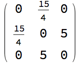
If None is used for the combiner, reciprocal edges are
not combined. A weighted multigraph is created instead.
IGWeightedUndirectedGraph[
Graph[{1 -> 2, 2 -> 1, 2 -> 3}, EdgeWeight -> {3, 4, 5}],
None
]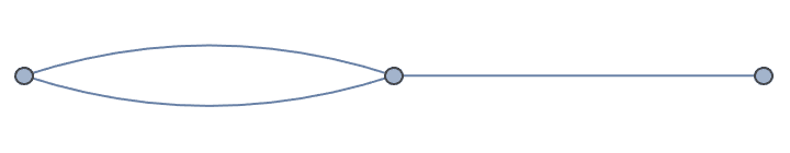
IGEdgeWeightedQ[%]True
?IGWeightedVertexDelete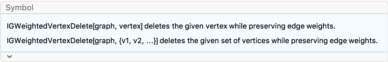
In Mathematica 11.3 and earlier, the built-in
VertexDelete does not handle edge weights correctly, and
may sometimes produce Graph expressions with a broken
internal structure. The purpose of IGWeightedVertexDelete
is to provide a fast and reliable way to remove a vertex while
preserving edge weights. Only edge weights are retained. All other
properties are discarded.
g = Graph[{1 <-> 2, 2 <-> 3},
EdgeWeight -> {4, 5}];IGEdgeProp[EdgeWeight][g]{4, 5}
IGEdgeProp[EdgeWeight]@IGWeightedVertexDelete[g, 3]{4}
Possible issues:
To delete a single vertex whose name is a list, it is necessary to
use the syntax IGWeightedVertexDelete[g, {v}] to avoid
ambiguity.
Graphs with list vertices commonly appear in the output of several
functions, such as NearestNeighborGraph,
RelationGraph, IGDisjointUnion or
IGMeshCellAdjacencyGraph.
g = NearestNeighborGraph[RandomInteger[4, {10, 2}],
VertexLabels -> "Name"] //
IGEdgeMap[Apply[EuclideanDistance], EdgeWeight -> EdgeList]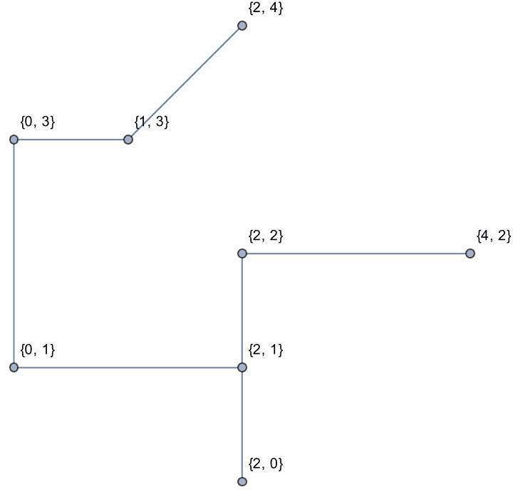
v = First@VertexList[g]{2, 2}
In this case, the single-vertex convenience syntax will not work.
IGWeightedVertexDelete[g, v]![]()
$Failed
Wrap the vertex in a list instead.
IGWeightedVertexDelete[g, {v}]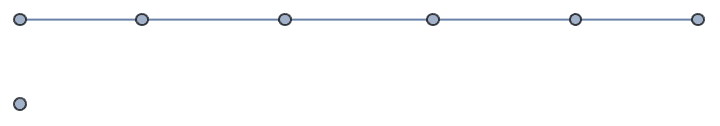
?IGWeightedSubgraph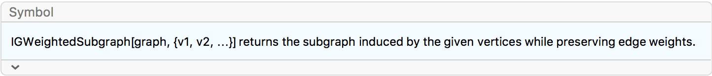
In Mathematica 11.3 and earlier, the built-in
Subgraph function does not preserve edge weights.
IGWeightedSubgraph preserves edge weights, but discards all
other properties.
To retain not only edge weights, but also other properties, use
IGTakeSubgraph. IGWeightedSubgraph offers much
better performance than IGTakeSubgraph at the cost of
discarding other properties.
g = Graph[{1 -> 2, 2 -> 3, 3 -> 4, 4 -> 1},
EdgeWeight -> {1, 2, 3, 4}, EdgeLabels -> "EdgeWeight",
VertexLabels -> "Name"]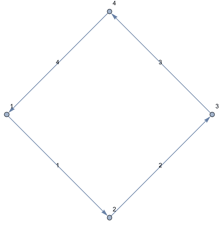
IGWeightedSubgraph[g, {2, 3, 4}, EdgeLabels -> "EdgeWeight",
VertexLabels -> "Name"]![]()
A sequence of integers is called graphical if there is an
undirected graph that has them as its degree sequence. Some authors
apply the term graphical only when the degrees can be realized
by a simple graph. Here we use it in a more general sense, as
IGraph/M is able to perform the test also for the cases of multigraphs
with loops, loop-free multigraphs and simple graph with at most one
self-loop per vertex. These are controlled by the SelfLoops
and MultiEdges options. The concept of graphicality
generalizes to pairs of in- and out-degree sequences of directed graphs
as well.
?IGGraphicalQ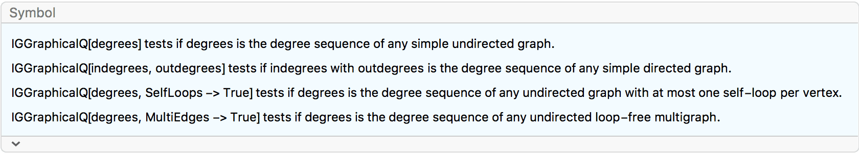
In the undirected case, IGGraphicalQ uses the
Erdős–Gallai theorem to check if the degree sequence is realized by any
simple graph. For loopy multigraphs, it is sufficient to check that the
sum of degrees is even. If self-loops are disallowed, there is the
additional condition that \(\sum _id_i\geq
d_{\max }\). If at most one self-loop is allowed per vertex, but
no multi-edges, a modification of the Erdős-Gallai conditions due to
Cairns and Mendan are used.
In the directed case, IGGraphicalQ uses the
Fulkerson–Chen–Antsee theorem with Berger’s refinement. For loopy
multi-digraphs, it is sufficient to check that the sum of in-degrees
equals the sum of out-degrees. If self-loops are disallowed, there is
the additional condition that the sum of in-degrees (or, alternatively,
the sum of out-degrees) is not smaller than the maximum total degree. If
at most one self-loop is allowed per vertex, but no multi-edges, the
problem becomes equivalent to realizability as a simple bipartite graph,
and the Gale–Ryser theorem can be used (see
IGBigraphicalQ).
To actually construct a realization, use the
IGRealizeDegreeSequence function. To sample random
realizations, use IGDegreeSequenceGame.
The allowed options are:
SelfLoops -> True checks if the degree sequence
has realizations that potentially contain self-loops.
MultiEdges -> True checks if the degree sequence
has realizations that potentially contain more than one connection
between pairs of vertices.
Check if a degree sequence is graphical …
IGGraphicalQ[{4, 3, 3, 2, 1, 1}]True
… then construct a realization as a simple graph:
IGRealizeDegreeSequence[{4, 3, 3, 2, 1, 1}]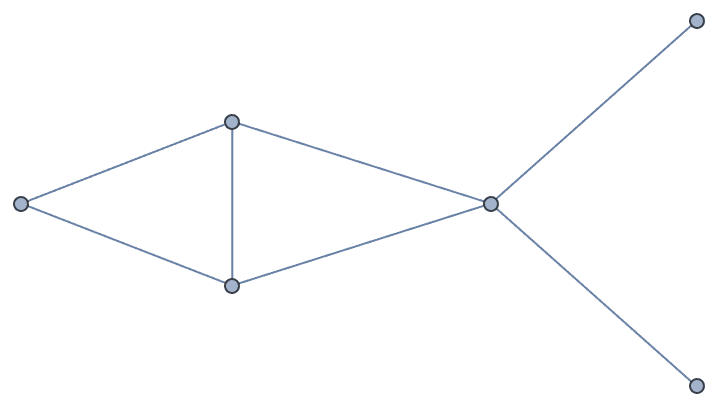
Check the same for a pair of in- and out-degree sequences, the construct a realization as a simple directed graph:
{IGGraphicalQ[{0, 2, 0}, {1, 0, 1}],
IGGraphicalQ[{1, 0, 1}, {0, 2, 0}]}{True, True}
{IGRealizeDegreeSequence[{0, 2, 0}, {1, 0, 1}],
IGRealizeDegreeSequence[{1, 0, 1}, {0, 2, 0}]}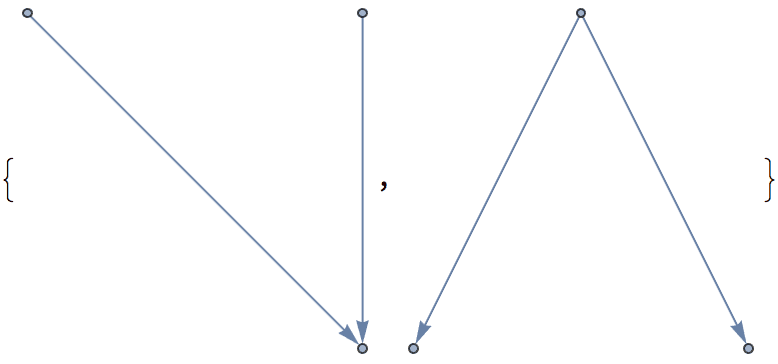
The degree sequence \((1,2,3)\) has
no realization as a simple graph, but it can be realized either as a
simple loopy graph,
![]() , or
as a loop-free multigraph,
, or
as a loop-free multigraph,
![]() .
.
{IGGraphicalQ[{1, 2, 3}],
IGGraphicalQ[{1, 2, 3}, SelfLoops -> True],
IGGraphicalQ[{1, 2, 3}, MultiEdges -> True]}{False, True, True}
\((4,1,1)\) is realizable as a loopy simple graph, but not as a loop-free multigraph.
{IGGraphicalQ[{4, 1, 1}, SelfLoops -> True],
IGGraphicalQ[{4, 1, 1}, MultiEdges -> True]}{True, False}
Any graph with the degree sequence \((6,2,2)\) must have both self-loops and multi-edges.
TableForm[
Outer[
IGGraphicalQ[{6, 2, 2}, SelfLoops -> #1, MultiEdges -> #2] &,
{False, True}, {False, True}
], TableHeadings -> {{"self-loops", "multi-edges"}, {"self-loops",
"multi-edges"}}]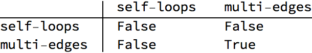
The following pair of in- and out-degree sequences can be realized as a directed graph with at most one self-loop per vertex, but not as a loop-free multigraph:
{IGGraphicalQ[{1, 0, 2}, {0, 1, 2}, SelfLoops -> True],
IGGraphicalQ[{1, 0, 2}, {0, 1, 2}, MultiEdges -> True]}{True, False}
Create a random graphical scale-free degree sequence and construct a corresponding graph:
ds = IGTryUntil[IGGraphicalQ]@
RandomVariate[ZipfDistribution[1.1], 100]{2, 14, 2, 1, 1, 2, 7, 1, 1, 1, 1, 1, 1, 11, 1, 1, 2, 1, 1, 3, 5, 1, \ 1, 1, 2, 9, 1, 1, 2, 7, 1, 1, 1, 1, 1, 5, 1, 1, 2, 2, 1, 1, 41, 2, 1, \ 3, 1, 1, 2, 3, 1, 1, 1, 1, 1, 1, 1, 1, 3, 2, 2, 1, 1, 1, 1, 4, 39, 1, \ 1, 4, 2, 4, 1, 1, 1, 3, 1, 1, 1, 1, 1, 14, 2, 2, 1, 1, 1, 1, 2, 10, \ 1, 1, 1, 4, 4, 1, 14, 2, 21, 7}
IGRealizeDegreeSequence[ds]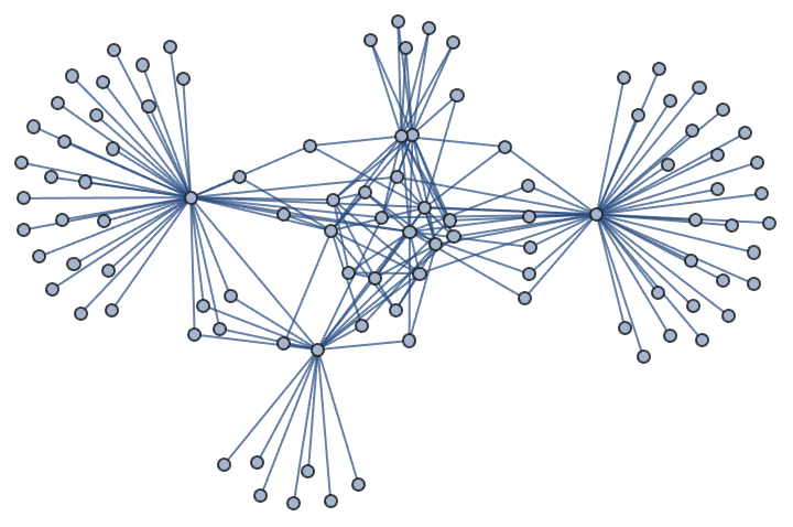
P. Erdős and T. Gallai, Gráfok Előírt Fokú Pontokkal, Matematikai Lapok 11, 264 (1960). https://users.renyi.hu/~p_erdos/1961-05.pdf
G. Cairns and S. Mendan, Degree Sequences for Graphs with Loops, 1 (2013). https://arxiv.org/abs/1303.2145v1
Z. Király, Recognizing Graphic Degree Sequences and Generating All Realizations, No. TR–2011–11, Egerváry Research Group, Eötvös Loránd University, 2012. http://bolyai.cs.elte.hu/egres/tr/egres-11-11.pdf
B. Cloteaux, Is This for Real? Fast Graphicality Testing, Computing in Science & Engineering 17, 6 (2015). https://dx.doi.org/10.1109/MCSE.2015.125
D. R. Fulkerson, Zero-One Matrices with Zero Trace, Pacific Journal of Mathematics 10, 3 (1960). https://doi.org/10.2140/pjm.1960.10.831
W. K. Chen, On the Realization of a \((p,s)\)-digraph with Prescribed Degrees, Journal of the Franklin Institute 281, 5 (1966). https://doi.org/10.1016/0016-0032(66)90301-2
R. P. Anstee, Properties of a Class of \((0,1)\)-matrices Covering a Given Matrix, Canadian Journal of Mathematics 34, 2 (1982). https://doi.org/10.4153/cjm-1982-029-3
A. Berger, A Note on the Characterization of Digraphic Sequences, Discrete Mathematics 314, 1 (2014). https://dx.doi.org/10.1016/j.disc.2013.09.010
Sz. Horvát and C. D. Modes, Connectivity matters: Construction and exact random sampling of connected graphs (2020). https://arxiv.org/abs/2009.03747
?IGBigraphicalQ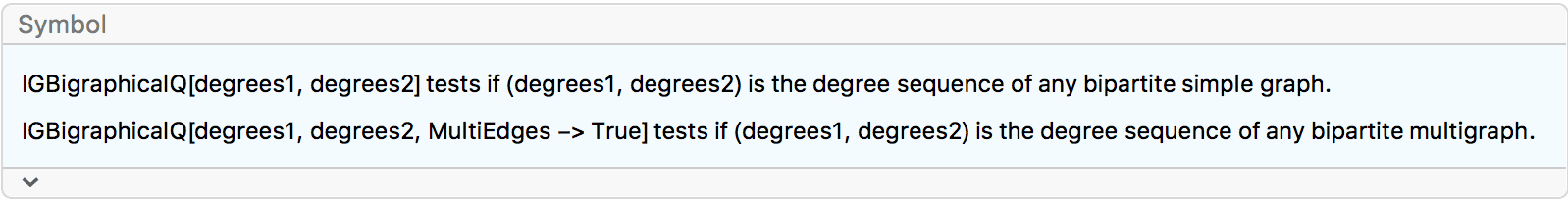
IGBigraphicalQ[degrees1, degrees2] checks if there is a
bipartite graph which has degrees1 and
degrees2 as the vertex degrees in the two partitions. Such
a pair of degree sequences is called bigraphical.
If multi-edges are allowed in the graph, it is sufficient to check
that the two degree sequences sum to the same value. If only simple
graphs are allowed, IGBigraphicalQ uses the Gale–Ryser
theorem with Berger’s refinement.
The available options are:
MultiEdges -> True allows for multi-edges in the
graph.IGBigraphicalQ[{4, 3, 1, 2, 4}, {2, 4, 4, 4}]True
The following pair of degree sequences is bigraphical only if multi-edges are permitted:
{IGBigraphicalQ[{2, 2}, {4}, MultiEdges -> False],
IGBigraphicalQ[{2, 2}, {4}, MultiEdges -> True]}{False, True}
H. J. Ryser, Combinatorial Properties of Matrices of Zeros and Ones, Can. J. Math. 9, 371 (1957). https://dx.doi.org/10.4153/cjm-1957-044-3
D. Gale, A theorem on flows in networks, Pacific J. Math. 7, 1073 (1957). https://dx.doi.org/10.2140/pjm.1957.7.1073
A. Berger, A Note on the Characterization of Digraphic Sequences, Discrete Mathematics 314, 1 (2014). https://dx.doi.org/10.1016/j.disc.2013.09.010
?IGPotentiallyConnectedQ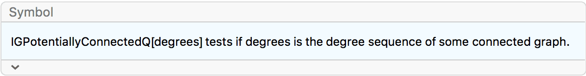
IGPotentiallyConnectedQ checks if a degree sequence has
a realization as a connected graph. The condition is that the degree
sequence \(\left(d_1,\ldots
,d_n\right)\) satisfy \(\frac{1}{2}\sum
_id_i\geq n-1\) and \(d_i>0\)
for all \(i\). Additionally,
IGPotentiallyConnectedQ requires that the sum of degrees be
odd.
Check the potential connectivity of a degree sequence, then construct a corresponding connected graph:
IGPotentiallyConnectedQ[{3, 2, 2, 1, 1, 1}]True
IGRealizeDegreeSequence[{3, 2, 2, 1, 1, 1}, Method -> "SmallestFirst"]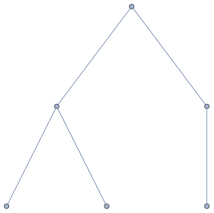
The empty degree sequence is considered non-potentially-connected:
IGPotentiallyConnectedQ[{}]False
The length-1 degree sequence \((0)\) is considered connected:
IGPotentiallyConnectedQ[{0}]True
IGPotentiallyConnectedQ returns False for
odd-sum sequences, as no graph can have them as its degrees:
IGPotentiallyConnectedQ[{3, 3, 3}]False
Generate a random potentially connected degree sequence and construct a corresponding connected non-simple graph:
IGRealizeDegreeSequence[
IGTryUntil[IGPotentiallyConnectedQ]@
RandomVariate[ZipfDistribution[1], 100],
MultiEdges -> True, SelfLoops -> True, Method -> "SmallestFirst"
]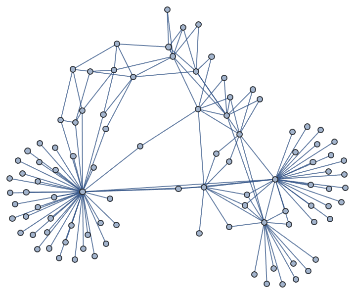
See the Graph creation section for a detailed description of these functions.
?IGRealizeDegreeSequence
?IGDegreeSequenceGame
?IGSplitQ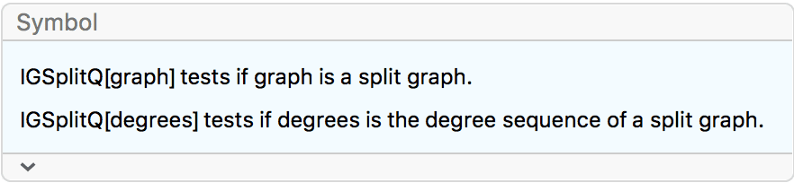
IGSplitQ recognizes split graphs, or their degree
sequences. Splits graphs are the graphs which can be partitioned into a
clique and an independent set. IGSplitQ ignores self-loops
and multi-edges.
Split graph can be recognized solely based on their degree sequence. Let \(d_1\geq d_2\geq \cdots \geq d_n\) be the non-increasingly ordered degree sequence, and \(m\) the largest index \(i\) such that \(d_i\geq i-1\). Then the graph is split if and only if
\[\sum _{i=1}^md_i=m(m-1)+\sum _{i=m+1}^nd_i.\]
When applied to a list of integers, IGSplitQ only checks
this condition, but does not verify graphicality.
Test if a graph is split:
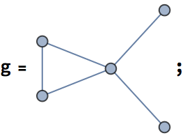
IGSplitQ[g]True
Highlight its clique and independent vertex set parts:
cl = First@IGLargestCliques[g];
HighlightGraph[g,
Subgraph[g, #] & /@ {cl, Complement[VertexList[g], cl]}]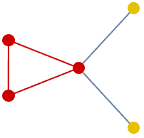
IGSplitQ can be used directly on degree sequences:
IGSplitQ@VertexDegree[g]True
The following graph is not split:
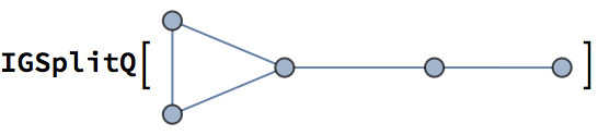
False
?IGThresholdQ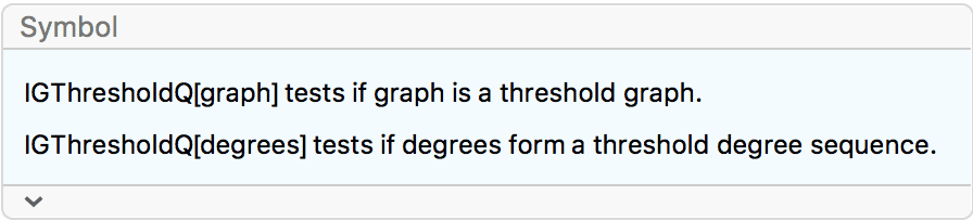
IGThresholdQ recognizes threshold graphs, or their
degree sequences. IGThresholdQ ignores self-loops and
multi-edges.
Check if the following is a threshold graph:
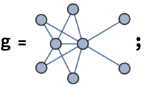
IGThresholdQ[g]True
Threshold graphs are also split graphs:
IGSplitQ[g]True
IGThresholdQ can be used directly on degree
sequences:
IGThresholdQ@VertexDegree[g]True
A threshold graph can be built by repeatedly adding either an
isolated vertex, or a dominating vertex, i.e. a vertex that connects to
all previous ones. The following function takes a specification in which
. and - represent isolated and dominating
vertices, respectively, and builds the corresponding graph.
thresholdGraph[spec_String] :=
With[{steps = Characters[spec]},
Graph[Range@Length[steps],
Join @@ Table[
If[steps[[i]] === "-",
UndirectedEdge[i, #] & /@ Range[i - 1], {}],
{i, Length[steps]}
]
]
]g = thresholdGraph["...--.-"]
IGThresholdQ[g]True
Degree sequences of threshold graphs have precisely one realization. Therefore, the same graph can be reconstructed from its degree sequence:
IGRealizeDegreeSequence@VertexDegree[g]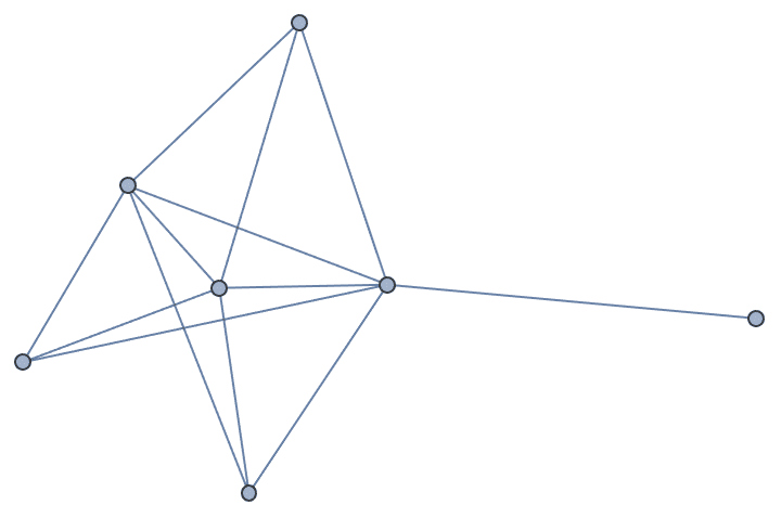
IGraph/M includes a set of functions that make it easy to extract
vertex and edge properties (attributes), transform them with an
arbitrary function, set their values based on the output of various
functions such as IGBetweenness, or to copy values from one
graph property into another.
To simplify these tasks, IGraph/M’s property handling framework takes
a somewhat more restrictive view of graph properties than
Mathematica’s built-ins. Edge and vertex properties are
strictly distinguished, and it is assumed that when a property exists
for one vertex (or edge), it also exists for all others. When this is
not the case, the value Missing["Nonexistent"] is used.
Let us use the following example network to demonstrate the basic usage of these functions.
g = Graph[ExampleData[{"NetworkGraph", "EastAfricaEmbassyAttacks"}],
ImageSize -> Medium]
?IGVertexPropertyList
?IGEdgePropertyList
Find what custom edge and vertex properties this graph has.
IGVertexPropertyList[g]{"FullName", "Group", VertexCoordinates, VertexLabels, VertexShape, \ VertexShapeFunction, VertexSize, VertexStyle}
IGEdgePropertyList[g]{EdgeShapeFunction, EdgeStyle, EdgeWeight}
?IGVertexProp
?IGEdgeProp
?IGEdgeVertexProp
Extract the "Group" property of each node:
IGVertexProp["Group"][g]{"Planners", "Planners", "Planners", "Planners", "Planners", \ "Planners", "Planners", "Planners", "Nairobi Cell", "Nairobi Cell", \ "Nairobi Cell", "Nairobi Cell", "Planners", "Dar es Salaam Cell", \ "Dar es Salaam Cell", "Dar es Salaam Cell", "Dar es Salaam Cell", \ "Dar es Salaam Cell"}
Extract the weight of each edge:
IGEdgeProp[EdgeWeight][g]{0.52, 0.36, 0.48, 0.48, 0.36, 0.36, 0.36, 0.36, 0.36, 0.16, 0.72, \ 0.16, 0.36, 0.36, 0.36, 0.36, 0.48, 0.36, 0.36, 0.48, 0.48, 0.48, \ 0.48, 0.48, 0.64, 0.48, 0.48, 0.48, 0.64, 0.48, 0.48, 0.48, 0.64, \ 0.28, 0.12, 0.48, 0.12, 0.12, 0.12, 0.12, 0.12, 0.64, 0.64, 0.48, \ 0.12, 0.64, 0.48, 0.48, 0.12, 0.12, 0.12}
?IGVertexMap
?IGEdgeMap
Show the value of the "FullName" custom property in
tooltips.
IGVertexMap[# &, Tooltip -> IGVertexProp["FullName"], g]
g = Graph[ExampleData[{"NetworkGraph", "EastAfricaEmbassyAttacks"}],
ImageSize -> Medium];Scale vertices according to degree:
IGVertexMap[0.1 # &, VertexSize -> VertexDegree, g]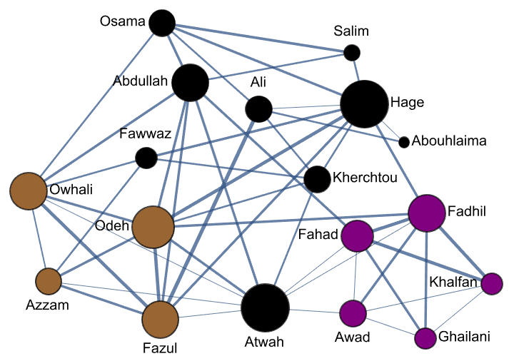
Let us colour edges by betweenness and set their thickness based on
weight. Betweenness calculations treat high weight values as a “long
distance”, thus we invert EdgeWeight before calculating the
betweenness. To be able to use the original weights, we save them into a
new "weight" property.
Calls to IGEdgeMap or IGVertexMap can be
conveniently chained together using their operator form.
g //
IGEdgeMap[ (* save original weight in "weight" property *)
Identity, "weight" -> IGEdgeProp[EdgeWeight]
]/*
IGEdgeMap[ (* invert edge weights for betweenness calculation *)
1/# &, EdgeWeight
]/*
IGEdgeMap[ (* thickness by original weight,
colour by betweenness based on inverse weight *)
Directive[AbsoluteThickness[9 #1], ColorData["Rainbow"][#2]] &,
EdgeStyle -> {IGEdgeProp["weight"],
Rescale@*EdgeBetweennessCentrality}
]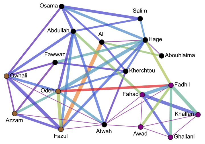
Label a graph with a circular layout:
IGVertexMap[
Function[{name, coord},
Placed[
name,
{{.5, .5}, -0.8 Normalize[coord] + {.5, .5}},
Rotate[#, Mod[ArcTan @@ coord, Pi, -Pi/2]] &
]
],
VertexLabels -> {VertexList, IGVertexProp[VertexCoordinates]},
IGLayoutCircle[ExampleData[{"NetworkGraph", "FamilyGathering"}]]
]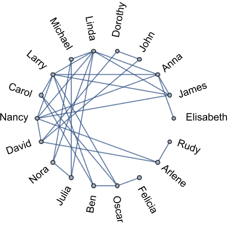
Use edge weights as edge labels, and line up labels with edges:
g = RandomGraph[{10, 20}, EdgeWeight -> RandomReal[1, 20]];(* returns edge angle for each edge *)
edgeAngle[g_] :=
With[{asc = AssociationThread[VertexList[g], GraphEmbedding[g]]},
ArcTan @@ (asc[#1] - asc[#2]) & @@@ EdgeList[g]
]IGLayoutDavidsonHarel[g] //
IGEdgeMap[
Function[{weight, angle},
Placed[
Style[NumberForm[weight, 2], Background -> White],
Center, Rotate[#, Mod[angle, Pi, -Pi/2]] &
]
],
EdgeLabels -> {IGEdgeProp@EdgeWeight, edgeAngle}
]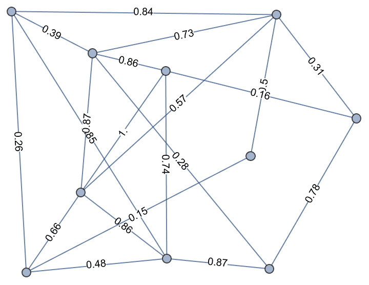
Colour vertices based on their graph distance form a given vertex:
g = ExampleData[{"NetworkGraph", "DolphinSocialNetwork"}];Graph[g, EdgeStyle -> LightGray, VertexSize -> 1,
ImageSize -> Medium] //
IGVertexMap[
ColorData["Rainbow"],
VertexStyle -> (Rescale@First@IGDistanceMatrix[#, {"Feather"}] &)
]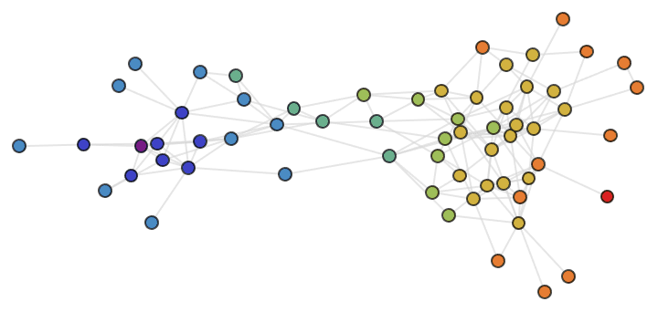
Colour the vertices of an annotated bipartite disease-gene graph based on whether they represent diseases or genes.
g = ExampleData[{"NetworkGraph", "BipartiteDiseasomeNetwork"}];There are two types of vertices:
IGVertexProp["Type"][g] // Union{"Disease", "Entrez"}
IGVertexMap[
<|"Disease" -> Red, "Entrez" -> Blue|>,
VertexStyle -> IGVertexProp["Type"],
g
]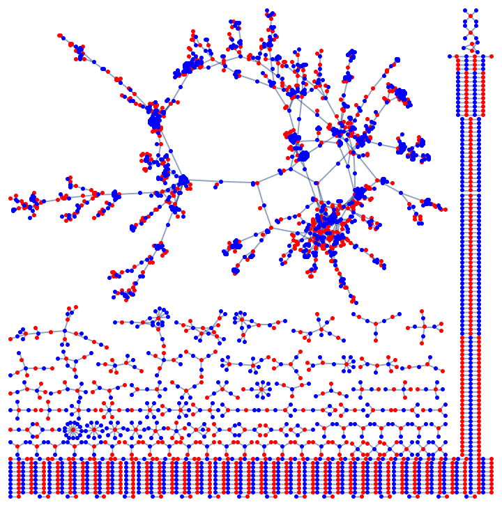
Compute the edge weights of a spatially embedded graph as lengths, then colour edges based on this value.
g = IGMeshCellAdjacencyGraph[
IGLatticeMesh["Pinwheel", Disk[{0, 0}, 4]], 2,
VertexCoordinates -> Automatic,
GraphStyle -> "ThickEdge", EdgeStyle -> Opacity[2/3]
]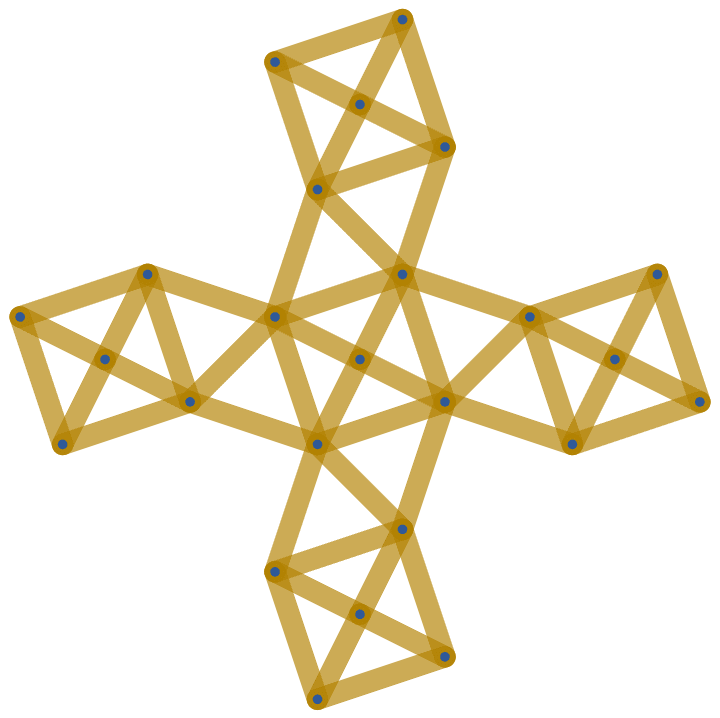
g //
IGEdgeMap[Apply[EuclideanDistance],
EdgeWeight -> IGEdgeVertexProp[VertexCoordinates]]/*
IGEdgeMap[ColorData["DarkRainbow"],
EdgeStyle -> Rescale@*IGEdgeProp[EdgeWeight]]
g = ExampleData[{"NetworkGraph", "FamilyGathering"}]
g = IGVertexMap[
Interpreter["GivenName"][#]["Gender"] &,
"gender" -> VertexList,
g
];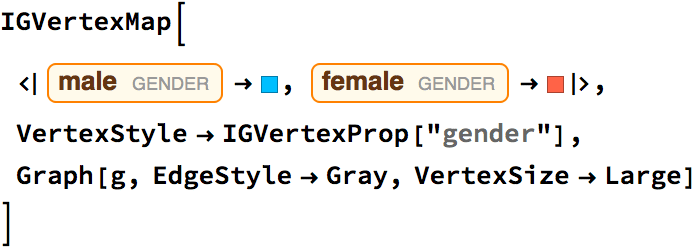
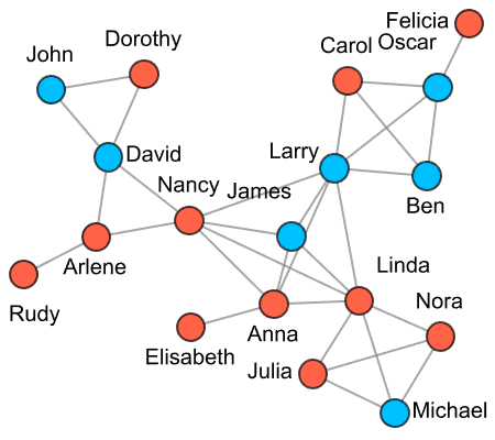
Transform the vertex coordinates of a graph to obtain a more pleasing layout:
g = Graph[GraphData[{"Apollonian", 5}, "EdgeList"],
GraphLayout -> "PlanarEmbedding"]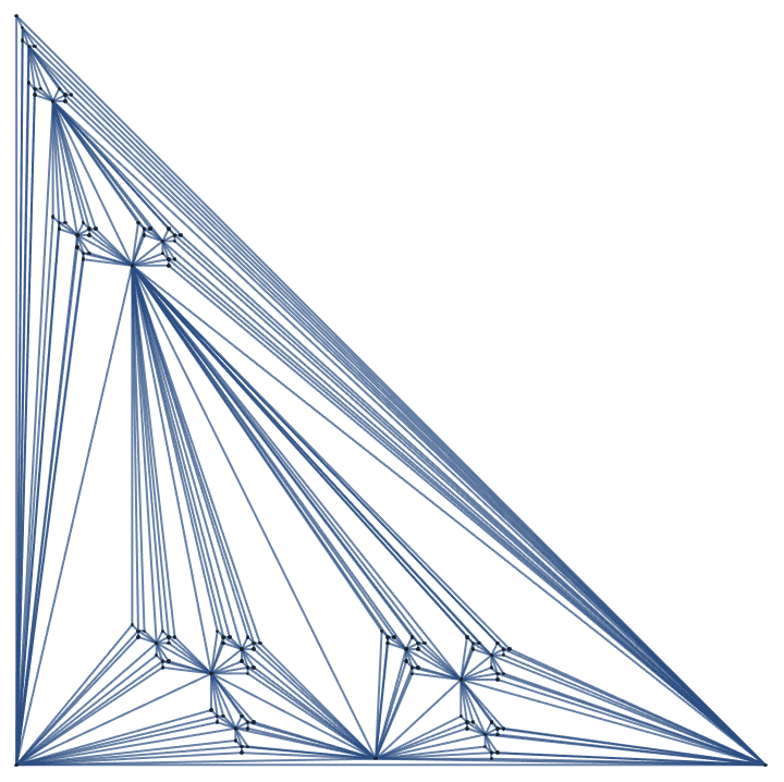
![]()
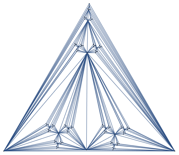
Project coordinates from the sphere to the plane using stereographic projection:
g = Graph3D[GraphData["DodecahedralGraph", "EdgeList"]]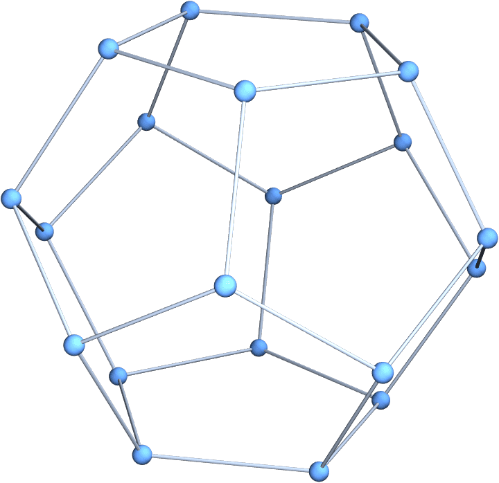
project =
CoordinateTransform[
{"Standard" -> "Stereographic", {"Sphere", 1}},
Rest@CoordinateTransform["Cartesian" -> "Spherical", #]
] &;Graph[
IGVertexMap[project,
VertexCoordinates -> Standardize@*IGVertexProp[VertexCoordinates],
g],
GraphLayout -> {"Dimension" -> 2}
]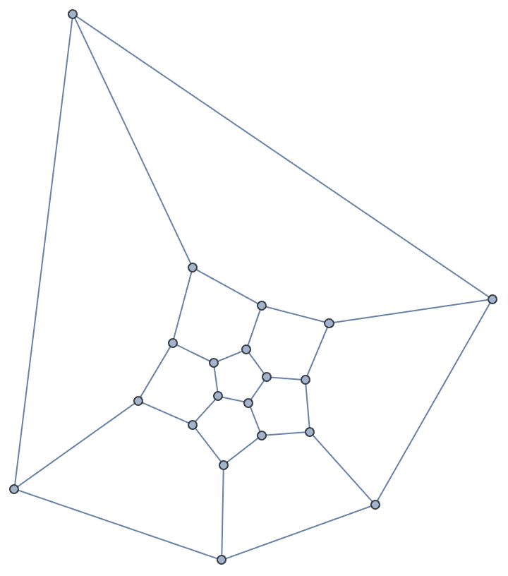
Let us import this network:
g = Import["http://networkdata.ics.uci.edu/data/lesmis/lesmis.gml",
ImageSize -> Large]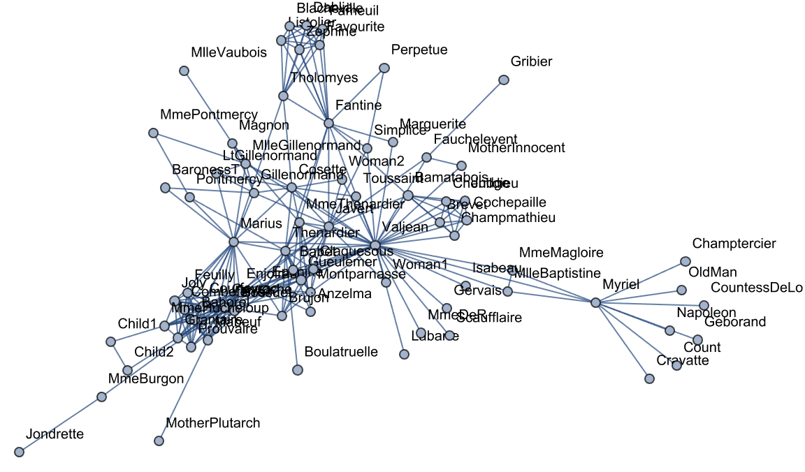
According to the description, this should be a weighted graph:
Import["http://networkdata.ics.uci.edu/data/lesmis/lesmis.txt"]"The file lesmis.gml contains the weighted network of coappearances \ of characters in Victor Hugo's novel \"Les Miserables\". Nodes \ represent characters as indicated by the labels and edges connect any pair of characters that appear in the same chapter of the book. The values \ on the edges are the number of such coappearances. The data on \ coappearances were taken from D. E. Knuth, The Stanford GraphBase: A Platform for Combinatorial Computing, Addison-Wesley, Reading, MA (1993)."
But as imported by Mathematica, it is not edge-weighted:
IGEdgeWeightedQ[g]False
This is because the edge weights are imported into the
"value" property instead of the standard
EdgeWeight:
IGEdgePropertyList[g]{"value", EdgeShapeFunction, EdgeStyle}
Copy the values of one property into another:
g = IGEdgeMap[# &, EdgeWeight -> IGEdgeProp["value"], g];Now we have a weighted graph:
IGEdgeWeightedQ[g]True
?IGKirchhoffMatrix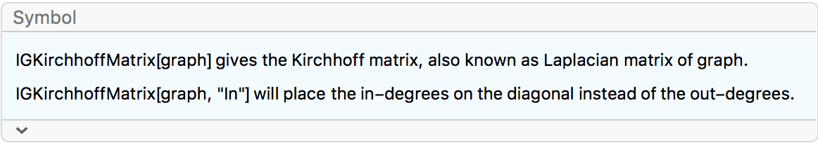
The Kirchhoff matrix of a graph is defined as
\[K_{i,j}= \begin{array}{ll} \{ & \begin{array}{ll} -a_{i,j}, \text{where }a_{i,j}\text{ is the number of }i\to j\text{ connections} & i\neq j \\ -\sum _{k\neq i}K_{k,i} & i=j \\ \end{array} \\ \end{array}\]
In other words, non-diagonal entries are the negative of the adjacency matrix and diagonal entries are equal to the out-degree. Rows sum up to zero.
The built-in KirchoffMatrix function uses the total
degree on the diagonal even if the input graph is directed, making it
unsuitable for many of the usual operations done with Kirchhoff
matrices.
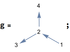
KirchhoffMatrix[g] // MatrixForm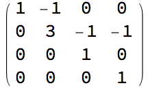
By default, the diagonal contains the out-degrees, and rows sum to
zero. This can also be requested explicitly using
IGKirchhoffMatrix[g, "Out"].
IGKirchhoffMatrix[g] // MatrixForm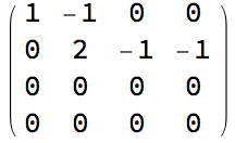
IGKirchhoffMatrix[g, "In"] will place the in-degrees on
the diagonal, so that the columns will sum to zero.
IGKirchhoffMatrix[g, "In"] // MatrixForm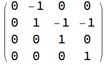
Unlike the built-in KirchhoffMatrix,
IGKirchoffMatrix takes into account edge
multiplicities.

![]()
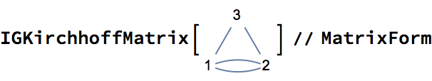
![]()
?IGJointDegreeMatrix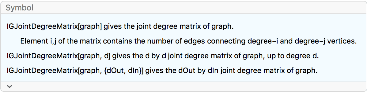
Entry \(J_{ij}\) of the joint degree matrix \(J\) is the number of edges connecting a degree \(i\) and a degree \(j\) vertex. For a directed graph, \(J_{ij}\) is the number of edges from a vertex with out-degree \(i\) to a vertex with in-degree \(j\).
For an empty (i.e. edgeless) graph, {{}} is
returned.
The available options are:
Normalized -> True will normalize the matrix by the
sum of entries for directed graphs. For undirected graphs, the sum of
upper triangular entries is used. Thus a matrix entry \(J_{ij}\) can be interpreted as the
probability that a randomly selected edge will connect vertices of
degrees \(i\) and \(j\).g = IGShorthand["1-2-3-4-2"]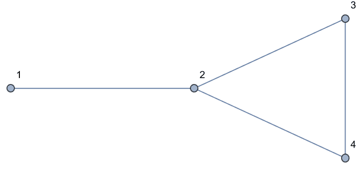
jdm = IGJointDegreeMatrix[g];
MatrixForm[jdm, TableHeadings -> Automatic]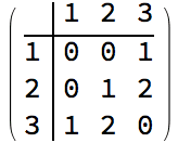
The degree distribution (excluding zero-degree nodes) can be recovered as follows. The result array contains the number of nodes having each degree.
![]()
{1, 2, 1}
Compute the degree distribution directly, for comparison.
Rest@BinCounts@VertexDegree[g]{1, 2, 1}
Some other systems use a slightly different definition of the joint degree matrix for undirected graphs: the number of degree \(i\) vertices connecting to degree \(j\) vertices. Compared to the definition used here, this definition counts edges running between nodes of the same degree twice. To obtain this type of joint degree matrix, simply add the diagonal to the original matrix.
MatrixForm[jdm + DiagonalMatrix@Diagonal[jdm],
TableHeadings -> Automatic]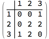
Multi-edges are supported.
![]()
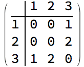
Self-loops are also supported. Note that
IGJointDegreeMatrix counts loop edges twice when computing
the vertex degree, just like VertexDegree. Thus the
vertices of the below graph have degrees 1 and 3.
![]()
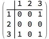
IGJointDegreeMatrix@
ExampleData[{"NetworkGraph", "ZacharyKarateClub"}] // MatrixPlot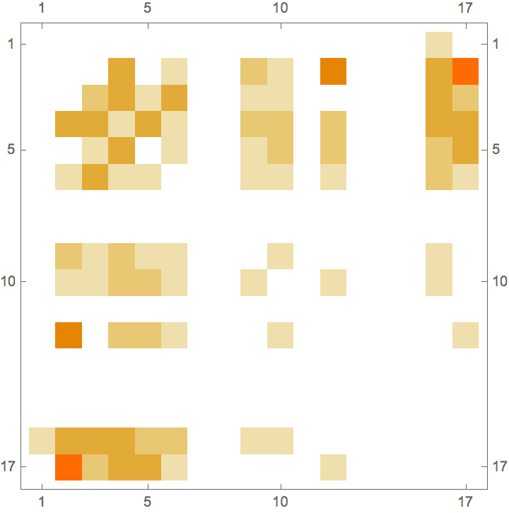
The joint degree matrix of a directed graph is not necessarily square.
IGBarabasiAlbertGame[15, 3] // IGJointDegreeMatrix // MatrixPlot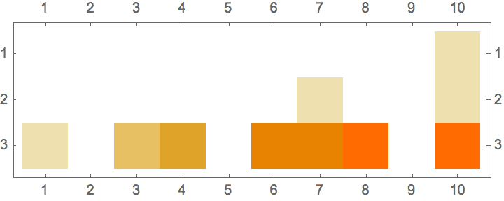
The second argument allows for obtaining joint degree matrices of a predictable size. This makes it convenient to operate together multiple joint degree matrices.
MatrixPlot@Mean@Table[
IGJointDegreeMatrix[RandomGraph[{10, 20}], 9, Normalized -> True],
{1000}
]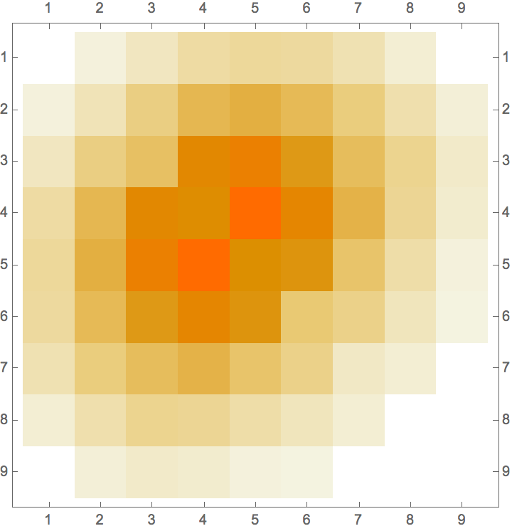
?IGAdjacencyMatrixPlot
IGAdjacencyMatrixPlot is based on
MatrixPlot, but optimized for the convenient display of
labelled adjacency matrices.
Available options:
EdgeWeight sets the edge property to use for matrix
elements. By default edge weights are used for weighted graphs. Set
EdgeWeight -> None to visualize the unweighted adjacency
matrix even for a weighted graph.
"UnconnectedColor" sets the colour to use to
represent non-existent connections.
VertexLabels controls how to label the matrix’s
columns and rows. Possible values:
"Index" uses row and column numbers. These are
identical to vertex indices when the full adjacency matrix is plotted,
but not when a partial matrix is plotted or if the vertices are
re-ordered.
"Name" uses vertex names.
Automatic uses indices for large graphs and names
for small ones. Use a list of rules to set different names for each
vertex.
"RotateColumnLabels" -> False will not rotate
columns labels.
Mesh controls the drawing of grid lines. By default,
a grid is drawn only for small graphs. Use Mesh -> All
to force drawing the grid.
IGAdjacencyMatrixPlot also accepts all standard
MatrixPlot options.
g = ExampleData[{"NetworkGraph", "Friendship"}]
IGAdjacencyMatrixPlot[g]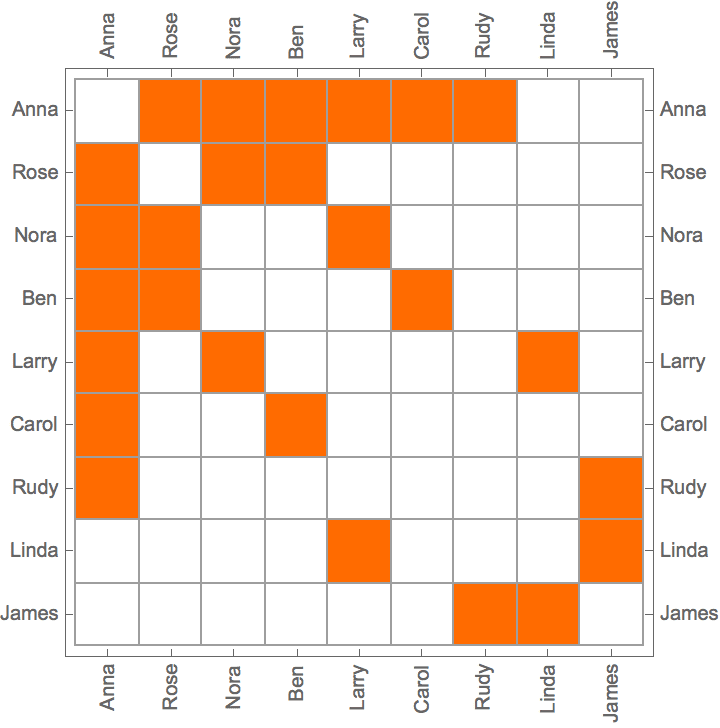
Reorder graph vertices before plotting.
IGAdjacencyMatrixPlot[g, Sort@VertexList[g]]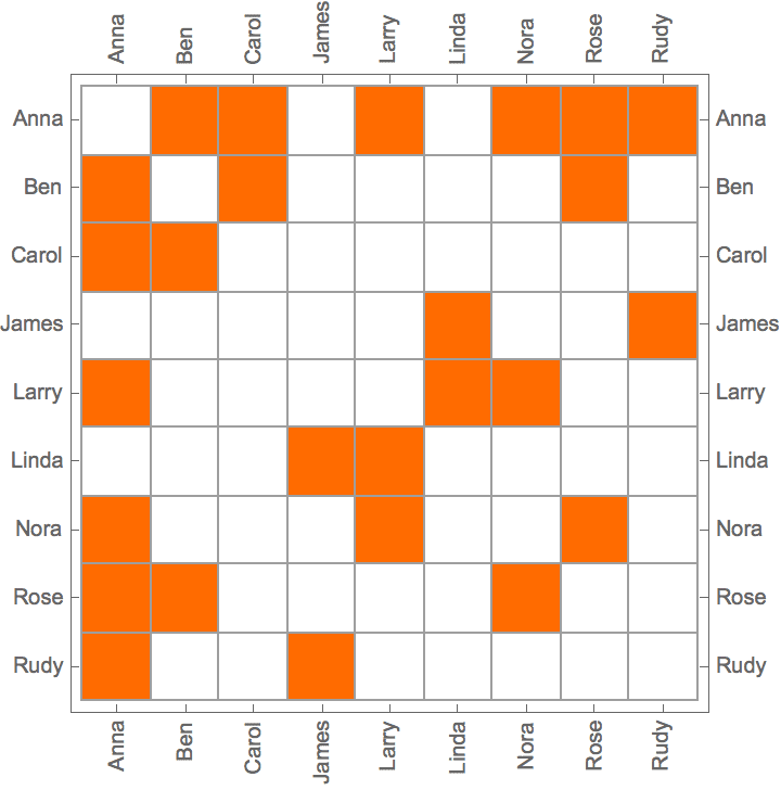
Plot a subgraph only.
IGAdjacencyMatrixPlot[g, {"Anna", "Ben", "Larry", "Carol"}]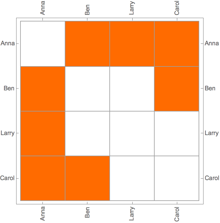
Plot a weighted adjacency matrix.
g = ExampleData[{"NetworkGraph", "EastAfricaEmbassyAttacks"}];
IGAdjacencyMatrixPlot[g, PlotLegends -> Automatic, ImageSize -> 300]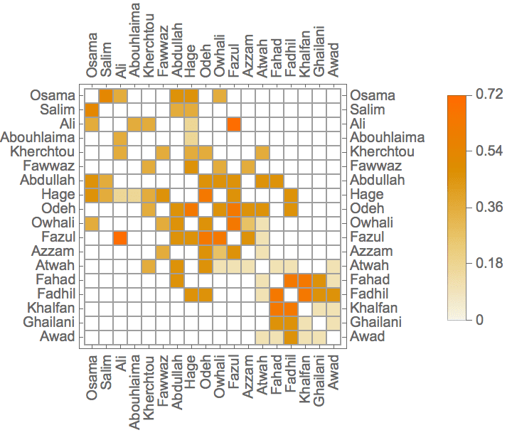
Use a different edge property than weights for the matrix entries.
g2 = g // IGEdgeMap[1/# &, EdgeWeight] //
IGEdgeMap[# &, "Betweenness" -> IGEdgeBetweenness];IGAdjacencyMatrixPlot[g2, EdgeWeight -> "Betweenness",
ImageSize -> 300]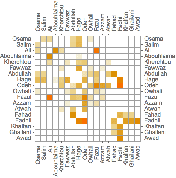
Control the style of matrix entries denoting the lack of a connection, to be able to distinguish them from zero entries.
IGAdjacencyMatrixPlot[g2, EdgeWeight -> "Betweenness",
"UnconnectedColor" -> Black, ImageSize -> 300]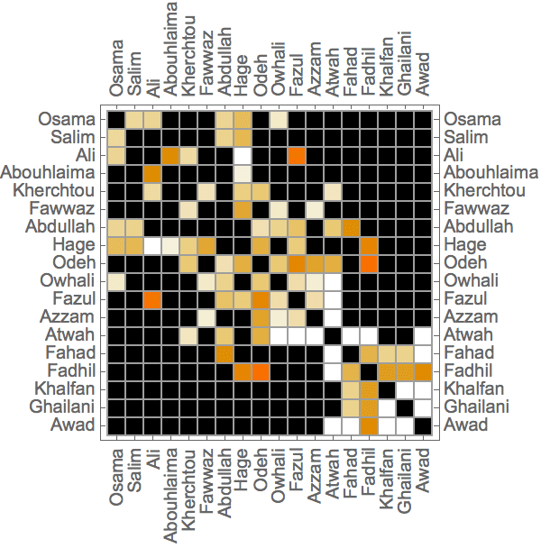
Plot the adjacency matrix of a very large network.
IGAdjacencyMatrixPlot[ExampleData[{"NetworkGraph", "PowerGrid"}]]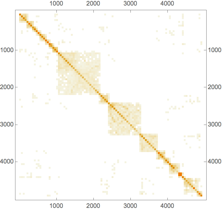
Large adjacency matrices, like the one above, are downsampled by
default to improve readability. This can be controlled using the
MaxPlotPoints option.
IGAdjacencyMatrixPlot[
ExampleData[{"NetworkGraph", "USPoliticsBooks"}],
MaxPlotPoints -> #] & /@ {Automatic, Infinity}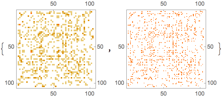
The vertex names and the grid are not shown by default for large graphs.
g = ExampleData[{"NetworkGraph", "DolphinSocialNetwork"}]
IGAdjacencyMatrixPlot[g]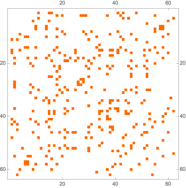
Force drawing vertex names and a grid regardless of the matrix size.
IGAdjacencyMatrixPlot[g, VertexLabels -> "Name", Mesh -> All,
ImageSize -> 440, FrameTicksStyle -> Tiny, MeshStyle -> Thin]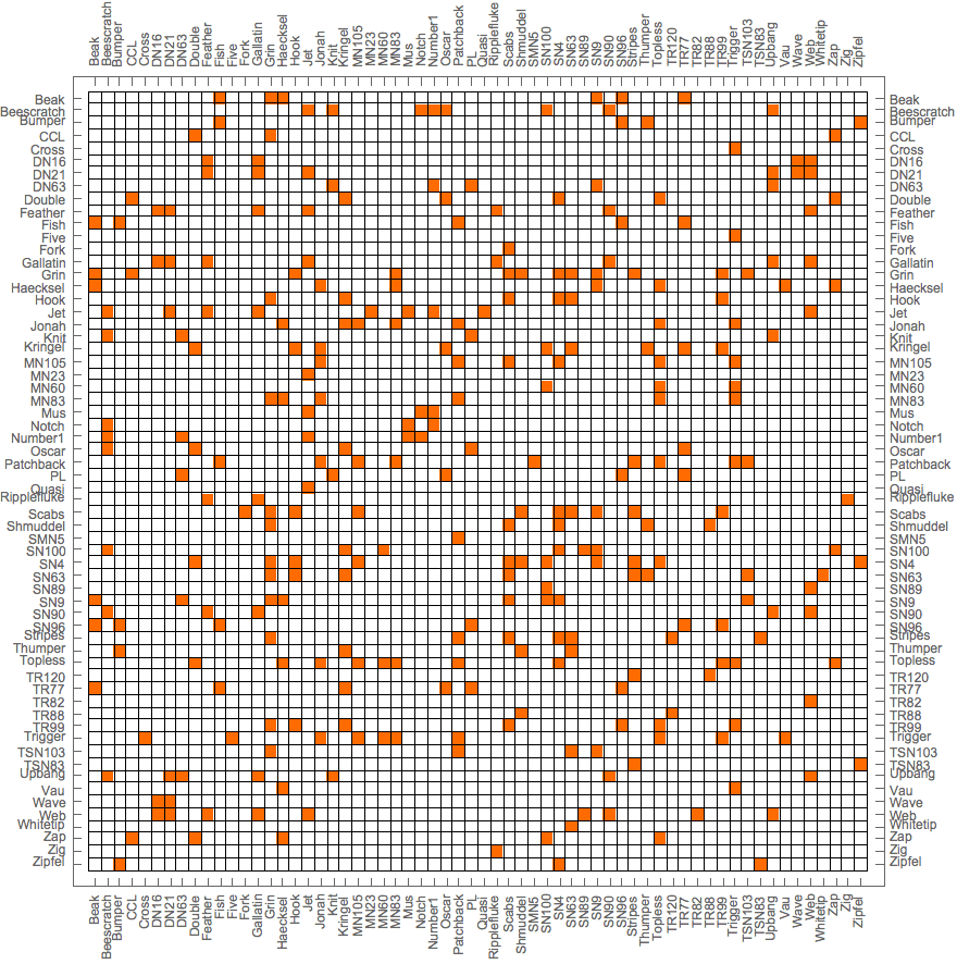
Reorder the adjacency matrix and draw grid lines to show community structure.
cl = IGCommunitiesEdgeBetweenness[g]![]()
IGAdjacencyMatrixPlot[g, Catenate@cl["Communities"],
Mesh -> ({#, #} &@FoldList[Plus, 0, Length /@ cl["Communities"]])]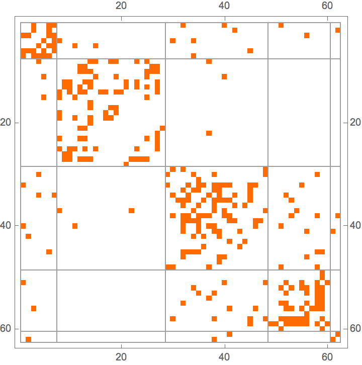
Avoid rotating vertex names when not necessary:
IGAdjacencyMatrixPlot[IGShorthand["A-B-C-D,A-C"],
"RotateColumnLabels" -> False]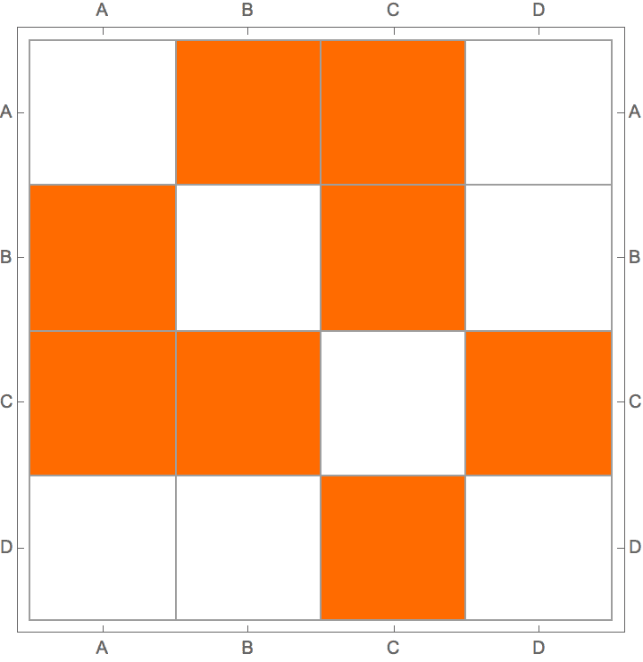
Use custom labels for vertices.
g = ExampleData[{"NetworkGraph", "SimpleFoodWeb"}]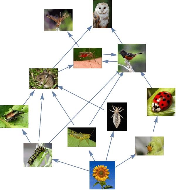
names = Thread[
VertexList[
g] -> (Show[#, ImageSize -> 20] & /@
IGVertexProp[VertexShape][g])]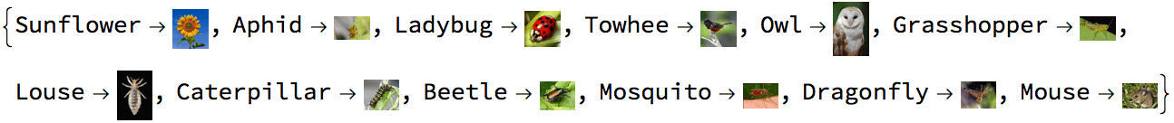
IGAdjacencyMatrixPlot[g, VertexLabels -> names,
"RotateColumnLabels" -> False, ImageSize -> Medium,
ColorRules -> {0 -> White, 1 -> Black}]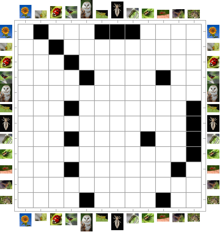
?IGZeroDiagonal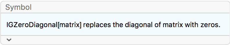
IGZeroDiagonal replaces the diagonal of a matrix with
zeros. It works on dense and sparse matrices, and supports non-square
matrices. This function is particularly useful when constructing
adjacency matrices that are to be converted to a graph.
mat = RandomReal[1, {6, 4}];IGZeroDiagonal[mat] // MatrixForm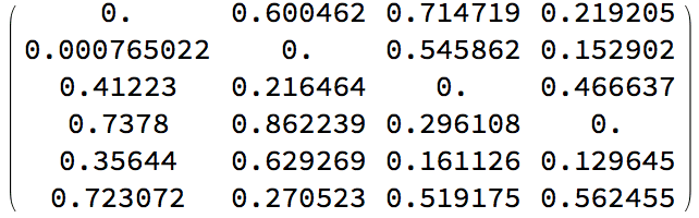
Connect those points in the plane whose Euclidean distance is less than 0.2, but do not connect each point with itself.
pts = RandomReal[1, {30, 2}];
AdjacencyGraph[
IGZeroDiagonal@UnitStep[0.2 - DistanceMatrix[pts]],
VertexCoordinates -> pts
]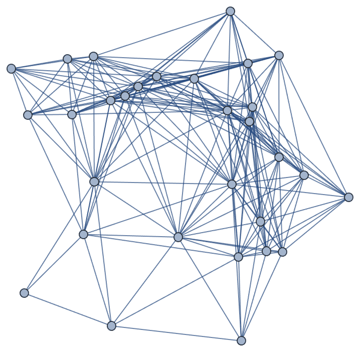
Connect each cell in a rectangular mesh to its Moore neighbours.
arr = RandomInteger[1, {10, 10}];
mesh = ArrayMesh[arr]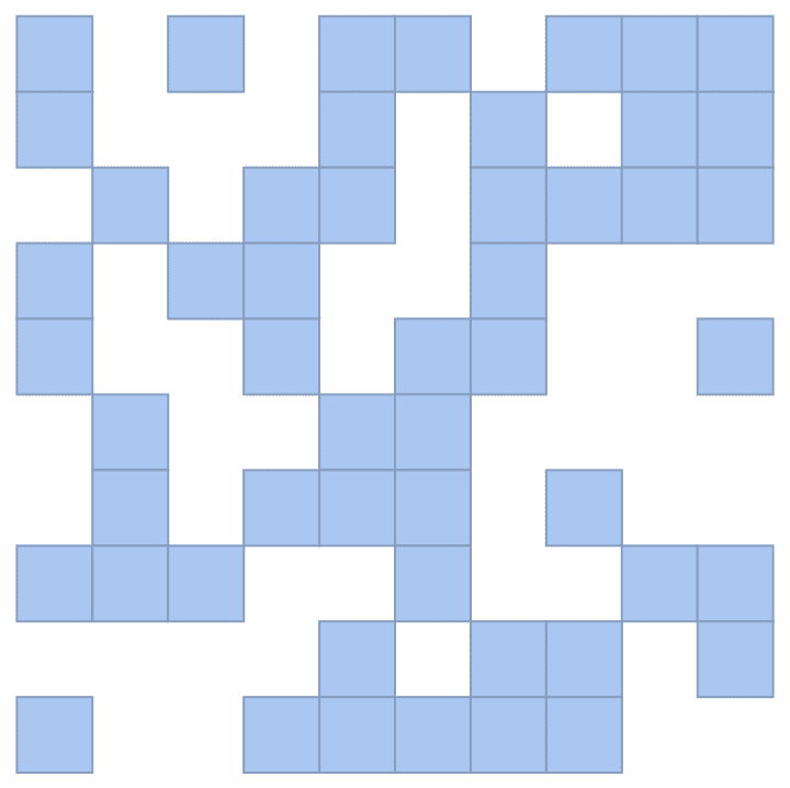
First, generate the square–vertex adjacency matrix.
mat = IGMeshCellAdjacencyMatrix[mesh, 2, 0]![]()
Then find the graph of squares adjacent through a corner point, but excluding self-adjacencies.
AdjacencyGraph[
IGZeroDiagonal@Unitize[mat . Transpose[mat]],
VertexCoordinates -> PropertyValue[{mesh, 2}, MeshCellCentroid],
GraphStyle -> "BasicBlack"
]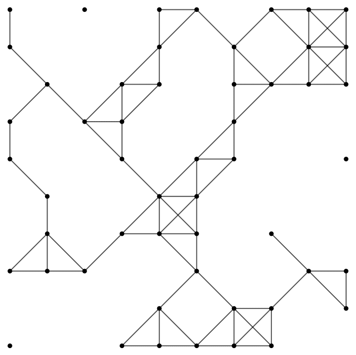
Show[mesh, %]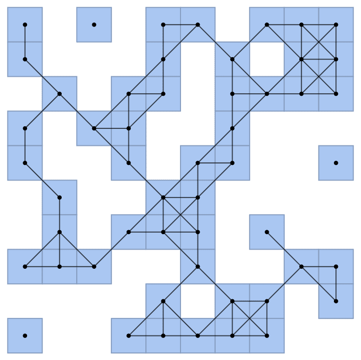
?IGTakeUpper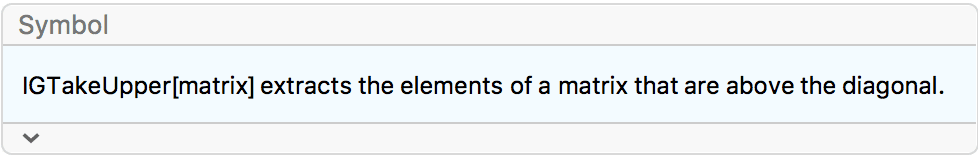
?IGTakeLower
IGTakeUpper and IGTakeLower extract the
above-diagonal and below-diagonal elements of a matrix. The matrix does
not need to be square. The elements are always extracted row-by-row.
mat = Partition[Range[16], 4];
MatrixForm[mat]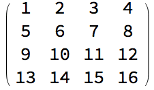
IGTakeUpper[mat]{2, 3, 4, 7, 8, 12}
IGTakeLower[mat]{5, 9, 10, 13, 14, 15}
IGTakeUpper and IGTakeLower support sparse
matrices. When given a sparse array as input, the result will also be a
sparse array.
sa = SparseArray[
RandomInteger[{1, 6}, {10, 2}] -> RandomInteger[10, 10]];
MatrixForm[sa]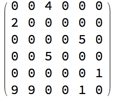
IGTakeUpper[sa]![]()
Normal[%]{0, 4, 0, 0, 0, 0, 0, 0, 0, 0, 5, 0, 0, 0, 1}
IGTakeUpper and IGTakeLower are optimized
for performance.
mat = RandomReal[1, {1000, 1000}];IGTakeUpper[mat]; // RepeatedTiming{0.000621611, Null}
Compute the mean pairwise distance of a random point set.
pts = RandomReal[1, {100, 2}];
Mean@IGTakeUpper@DistanceMatrix[pts]0.353733
IGraph/M provides importers and exporters for certain graph formats.
?IGImport
?IGImportString
Importing is done using IGImport and
IGImportString, which work analogously to the built-in
Import and ImportString. The supported export
formats are listed in $IGImportFormats:
$IGImportFormats{"Graph6"}
The Graph6, Sparse6 and Digraph6 formats are used by the
gtools suite included with nauty. IGraph/M
refers to this family of formats collectively as the “Nauty formats”.
gtools includes many command line programs for generating,
transforming and filtering graphs. For more information about
gtools, see http://pallini.di.uniroma1.it/
The formal description of these formats is available on the home page of Brendan McKay at https://users.cecs.anu.edu.au/~bdm/data/formats.html.
As of version 12.1, Mathematica has built-in support for Graph6 and Sparse6, but not for Digraph6. IGraph/M provides support Digraph6, a unified interface to all three formats (with auto-detection of the specific sub-format), as well as significantly better performance.
To convert a single string to a graph, use
IGFromNauty.
IGFromNauty["JR_IK?@?I?_"]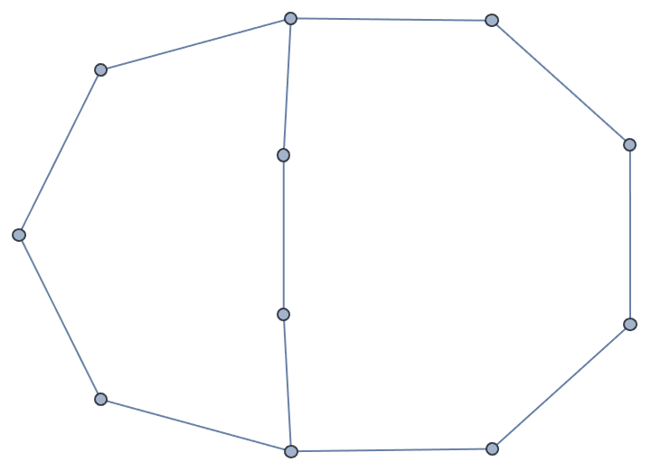
The purpose of IGImport and IGImportString
is to read lists containing several graphs.
IGImportString["
G]kq]K
G]dq\\S
G]Ku]W
G[|akk
GS\\unO
G~`HW{", "Graph6"]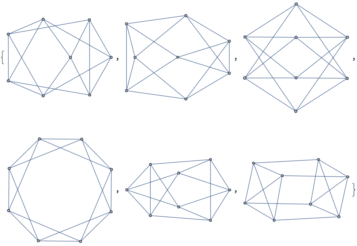
The following examples assume that the gtools programs
are in a directory that is on the operating system’s PATH environment
variable. If necessary, specify the full path to each program.
Generate all non-isomorphic undirected graphs on 4 vertices.
IGImport["!geng 4", "Nauty"]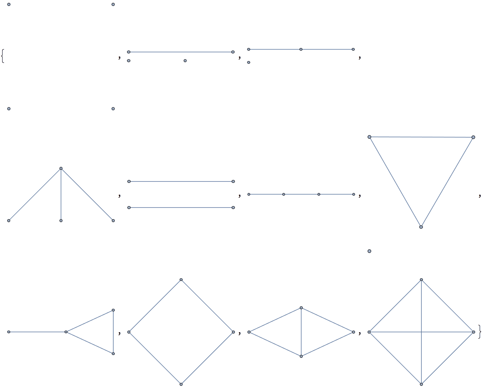
Generate all non-isomorphic directed graphs on 3 vertices.
IGImport["!geng 3 | directg", "Graph6",
GraphLayout -> "CircularEmbedding"]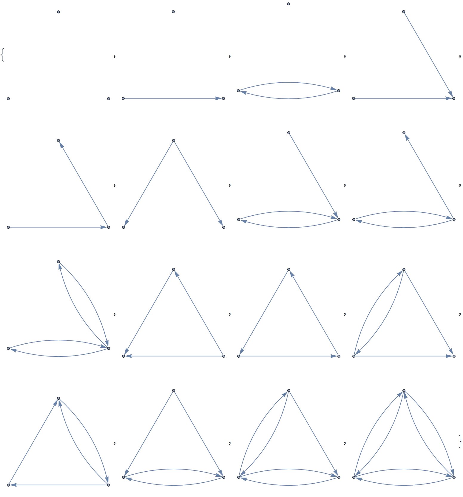
Find all non-isomorphic cactus graphs on 5 vertices. A cactus on
\(V\) vertices has between \(V-1\) and \(3
(V-1)/2\) edges. Thus we instruct the geng program
to only generate connected graphs with an edge count in this range.
Select[
IGImport["!geng -c 5 4:6", "Graph6", GraphStyle -> "Minimal"],
IGCactusQ
]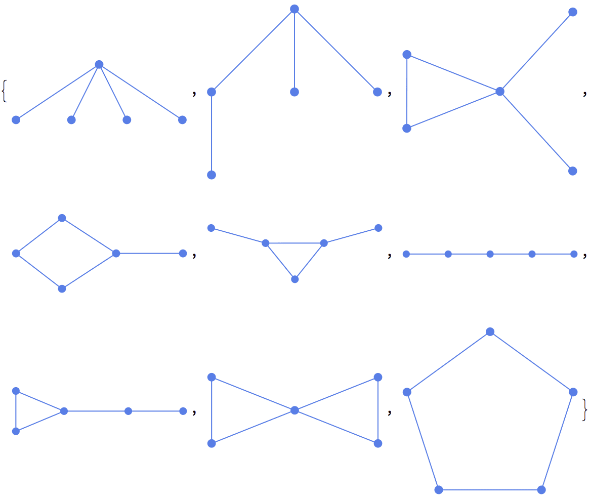
Generate all strongly connected tournaments on 5 vertices.
IGImport["!gentourng -c 5 -z", "Graph6"]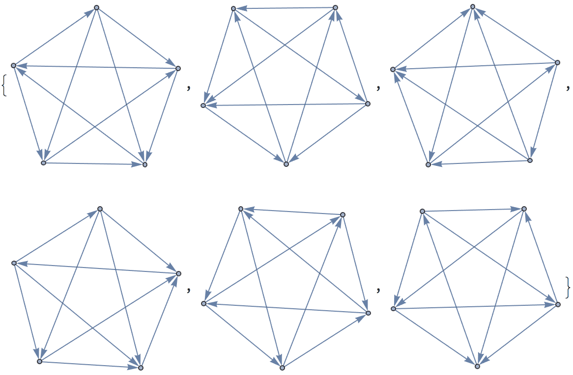
Generate all non-isomorphic trees on 6 vertices.
gengtreeg outputs Sparse6 by default. IGImport
detects this format automatically.
IGImport["!gentreeg 6", "Nauty", GraphStyle -> "WarmColor"]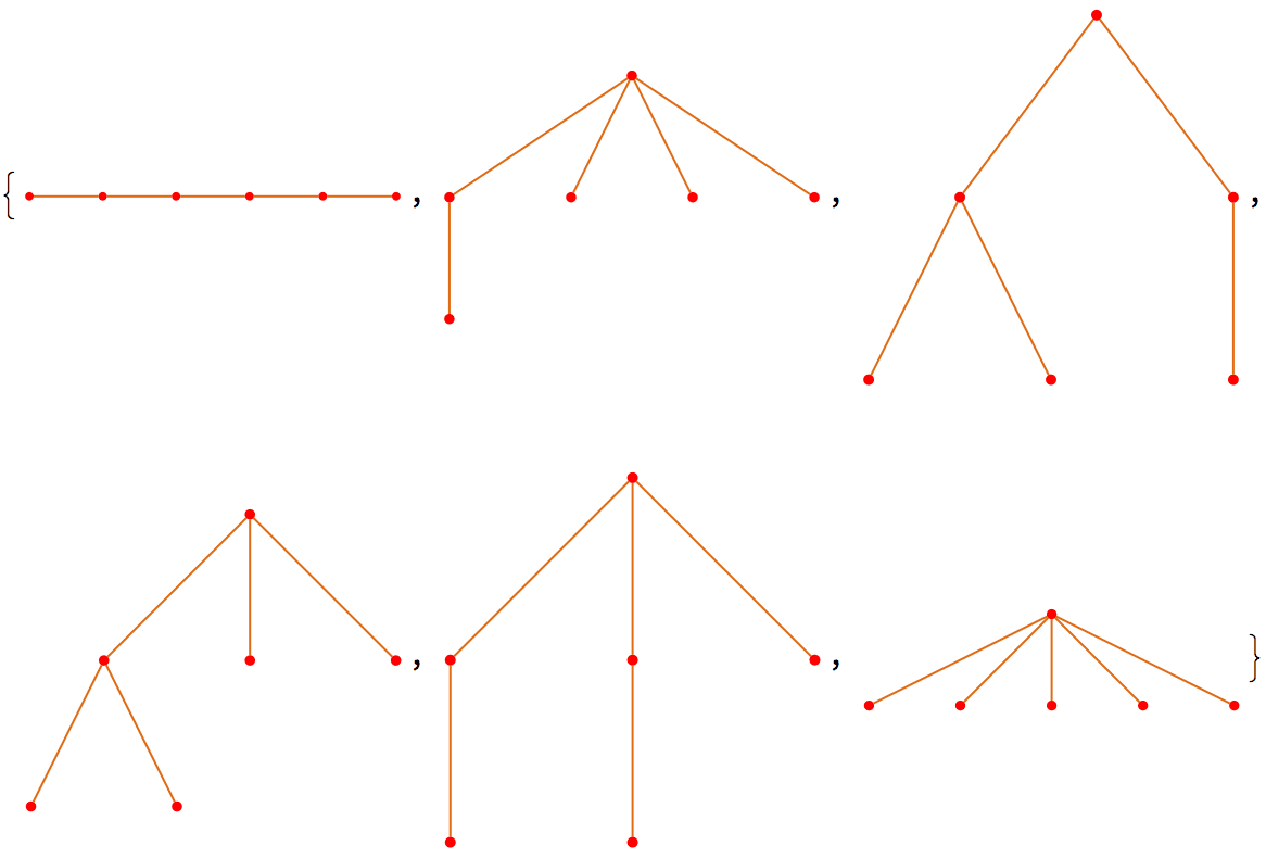
?IGExport
?IGExportString
Exporting is done using IGExport and
IGExportString, which work analogously to the built-in
Export and ExportString. The supported export
formats are listed in $IGExportFormats:
$IGExportFormats{"GraphML"}
As of Mathematica 13.0, the built-in Export
function produces non-standard GraphML files that cannot be read by some
other graph manipulation packages, such as the igraph library itself.
IGExport provides a standards-compliant implementation.
IGExportString[
ExampleData[{"NetworkGraph", "EurovisionVotes"}],
"GraphML"
] // Short[#, 15] & (* avoid showing more than 15 lines *)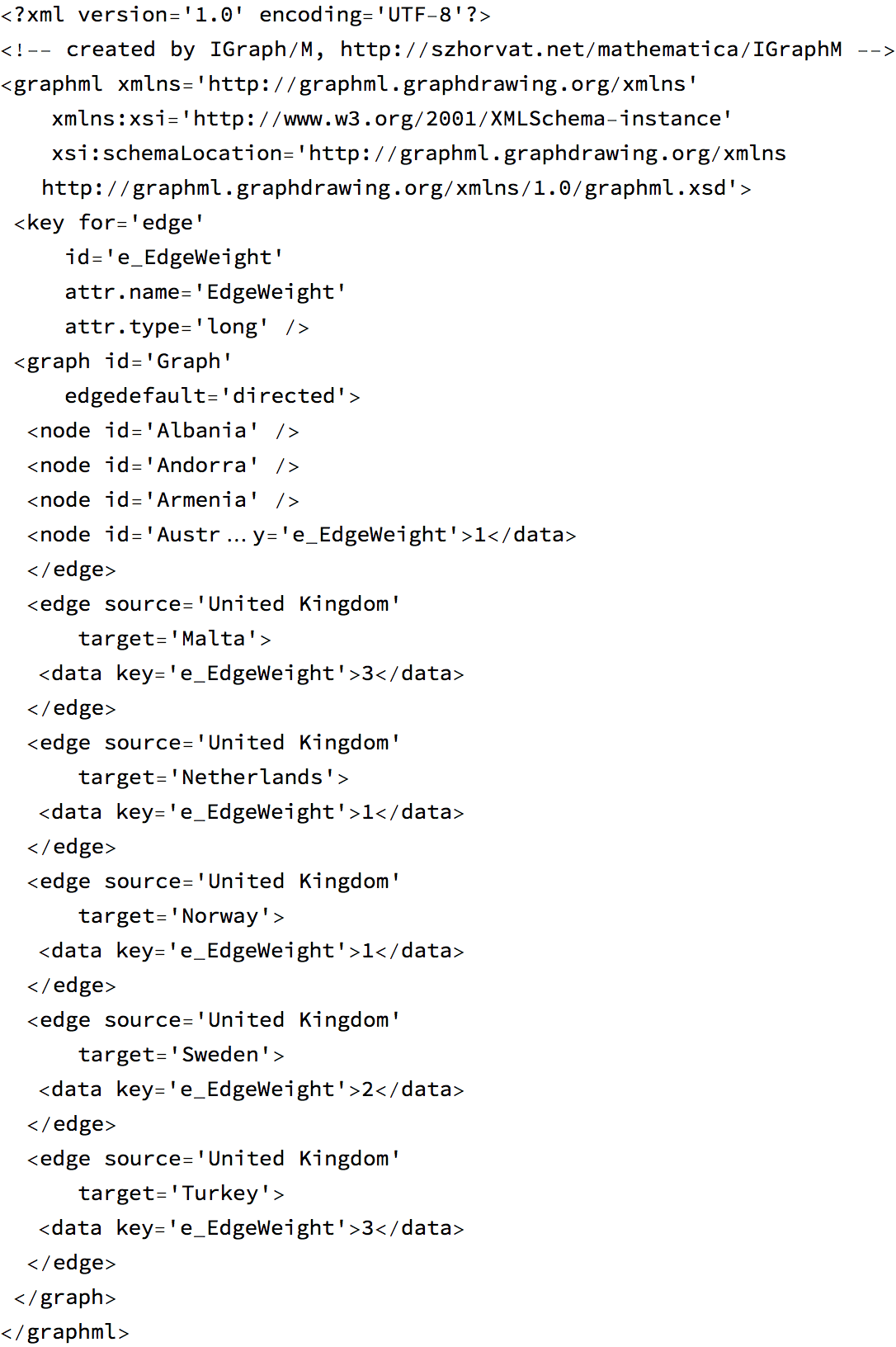
?IGUndirectedGraph
IGUndirectedGraph[g, method] converts a directed graph
to an undirected one, using the specified edge conversion method:
"Simple" creates a single undirected edge between
connected vertices
"All" creates one undirected edge for each directed
one. This may result in multiple edges between the same
vertices.
"Mutual" creates an edge only between mutually
connected vertices.
If the graph was already undirected, it will not be changed.
IGUndirectedGraph is guaranteed to preserve both the
vertex names and the vertex ordering of the original graph. The built-in
UndirectedGraph has a bug where it sometimes relabels
vertices.
Warning: As of IGraph/M 0.5,
IGUndirectedGraph discards graph properties such as edge
weights.
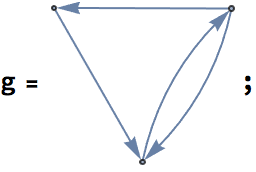
IGUndirectedGraph[g, #] & /@ {"Simple", "All", "Mutual"}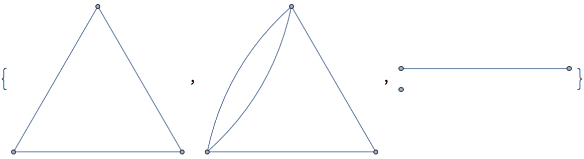
The default method is "Simple":
IGUndirectedGraph[g]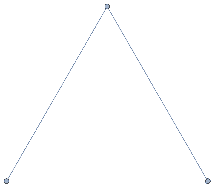
Self-loops are preserved by all methods:
IGUndirectedGraph[Graph[{1, 2}, {1 -> 1, 1 -> 2}], #] & /@ {"Simple",
"All", "Mutual"}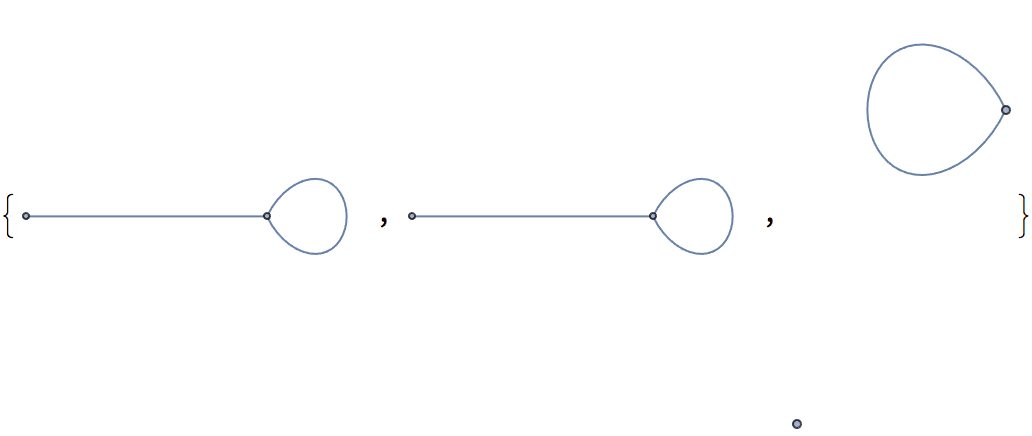
?IGReverseGraph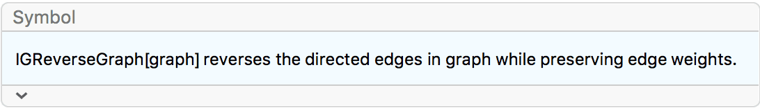
In Mathematica 11.3 and earlier, ReverseGraph
does not correctly transfer graph properties such as edge weights to the
result.
IGReverseGraph reverses the direction of each edge while
preserving the following graph properties: EdgeWeight,
EdgeCapacity, EdgeCost,
VertexWeight, VertexCapacity. Other properties
are discarded.
Undirected graphs are returned unmodified.
?IGSimpleGraph
IGSimpleGraph removes self-loops and collapses
multi-edges into simple ones, as specified in the options.
The available options are:
SelfLoops -> True keeps self-loops in the
graph.
MultiEdges -> True keeps parallel edges in the
graph.
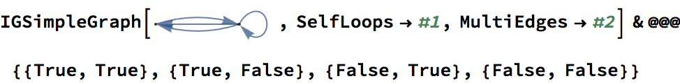

?IGDisjointUnion
IGDisjointUnion will combine the given graphs into a
single graph having them as its connected components.
IGDisjointUnion differs from the built-in
GraphDisjointUnion in several ways.
IGDisjointUnion takes the input graphs in a list instead
of as separate arguments. It can also take graph options to apply to the
final graph.
![]()
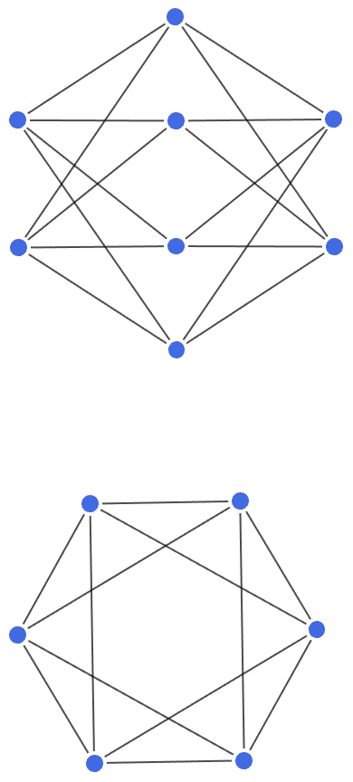
IGDisjointUnion is considerably faster than
GraphDisjointUnion when combining moderately sized
networks.
graphs = RandomGraph[{300, 600}, 30];IGDisjointUnion[graphs]; // RepeatedTiming{0.0125693, Null}
GraphDisjointUnion @@ graphs; // RepeatedTiming{0.529968, Null}
IGDisjointUnion does not support mixed graphs.
IGDisjointUnion[{Graph[{1 <-> 2}],
Graph[{1 \[DirectedEdge] 2}]}]![]()
$Failed
Use GraphDisjointUnion instead.
GraphDisjointUnion[Graph[{1 <-> 2}],
Graph[{1 \[DirectedEdge] 2}]]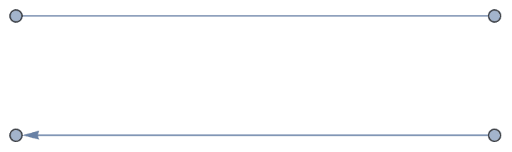
IGDisjointUnion will use vertex names of the form
{gi, v}, where gi is an identifier of the
original graph and v is the original name of the vertex.
When the input is a list gi is the index of the original
graph. When the input is an association, gi is its key.
In contrast, GraphDisjointUnion uses consecutive
integers as vertex names. Use IndexGraph to obtain a
similar result from the output of IGDisjointUnion.
g = IGDisjointUnion[<|"a" -> CycleGraph[4], "b" -> StarGraph[4]|>];
VertexList[g]{{"a", 1}, {"a", 2}, {"a", 3}, {"a", 4}, {"b", 1}, {"b", 2}, {"b", 3}, {"b", 4}}
This allows for convenient further manipulation, or for copying over arbitrary properties stored in the original graphs.
Graph[g, VertexStyle -> {{"a", _} -> Green, {"b", _} -> Red}]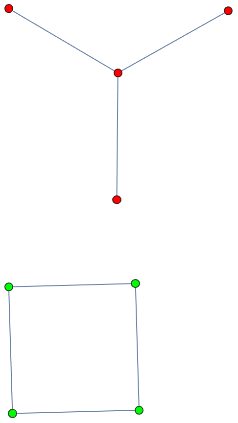
graphs = {
Graph[{Property[1 -> 2, "length" -> 5]}],
Graph[{Property[1 -> 2, "length" -> 3],
Property[3 -> 2, "length" -> 2]}]
};
IGDisjointUnion[graphs,
Properties -> {{gi_, v1_} \[DirectedEdge] {gi_, v2_} :> {"length" ->
PropertyValue[{graphs[[gi]], v1 \[DirectedEdge] v2},
"length"]}}]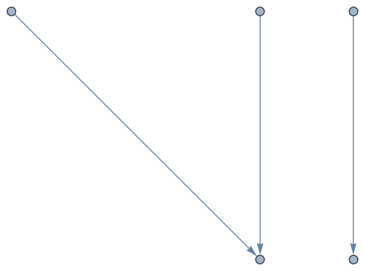
IGEdgeProp["length"][%]{5, 3, 2}
IGDisjointUnion is also practically useful for simply
showing many small graphs together.
IGDisjointUnion[
Select[IGGraphAtlas /@ Range[2, 150], IGConnectedQ],
GraphStyle -> "BasicBlue", VertexSize -> 1
]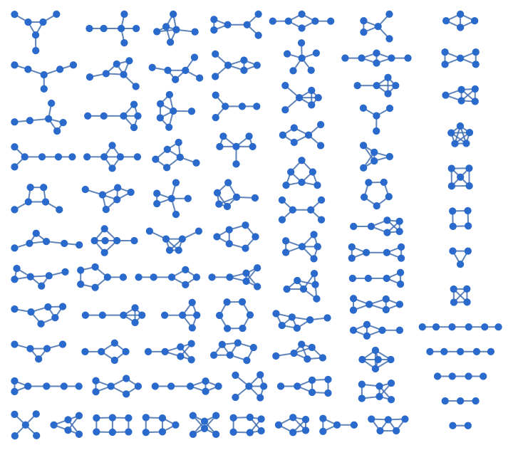
g = IndexGraph[%]; (* workaround for highlighting in Mathematica \
<= 11.2 *)
HighlightGraph[IGLayoutFruchtermanReingold[g],
ConnectedGraphComponents[g]]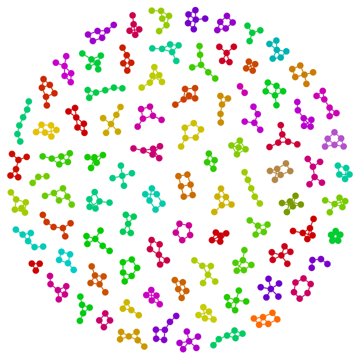
?IGOrientTree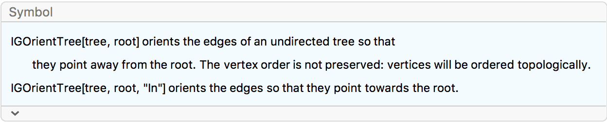
IGOrientTree creates an out-tree (also called an
arborescence) out of an undirected tree. Graph properties are preserved,
but the vertex ordering of the graph is changed.
g = KaryTree[10, 3, VertexLabels -> "Name"]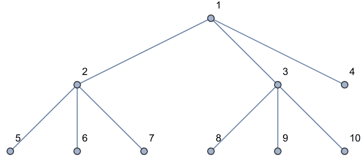
IGOrientTree[g, 1]
IGOrientTree[g, 5, GraphLayout -> "LayeredDigraphEmbedding"]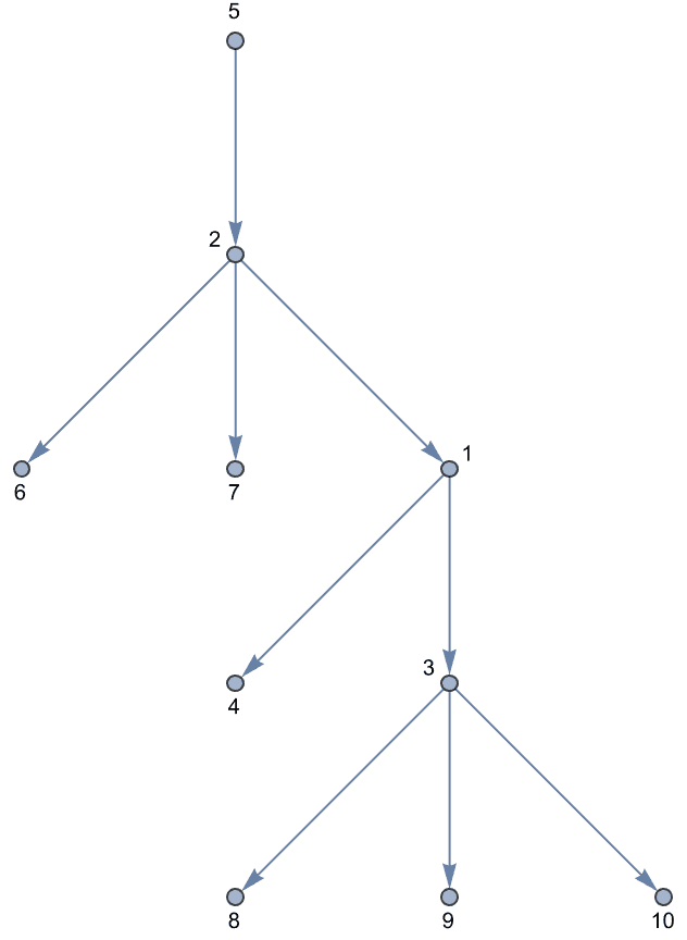
The result is an out-tree, also called an arborescence.
IGTreeQ[%, "Out"]True
Once the tree is made directed, it is easy to find its root and leaf nodes:
{IGSourceVertexList[%], IGSinkVertexList[%]}{IGSourceVertexList[True], IGSinkVertexList[True]}
Edges can be oriented towards or away from the root.
t = IGTreeGame[7, VertexLabels -> Automatic]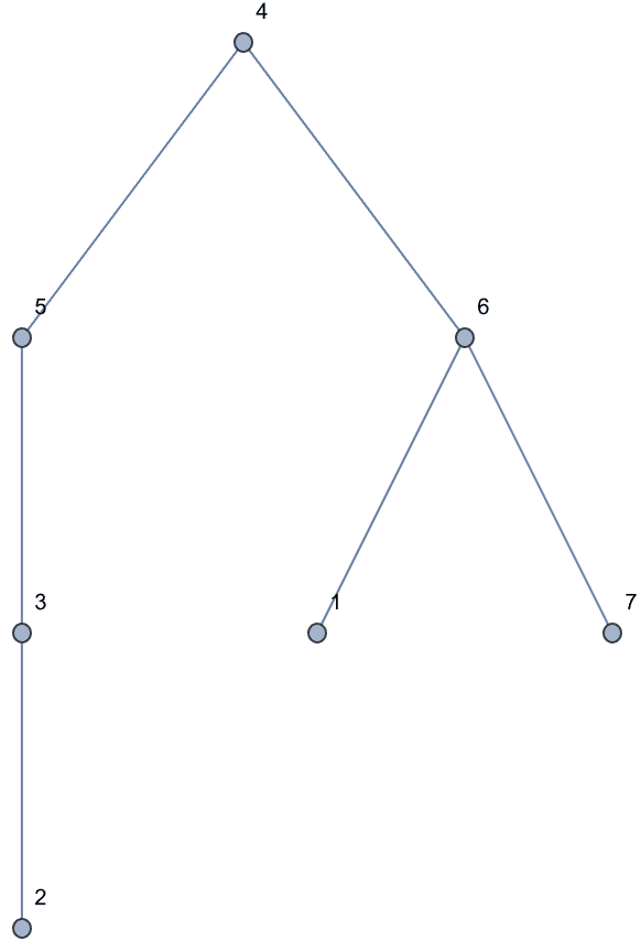
IGOrientTree[t, 4, #,
GraphLayout -> {"LayeredEmbedding", "RootVertex" -> 4}] & /@ {"In",
"Out"}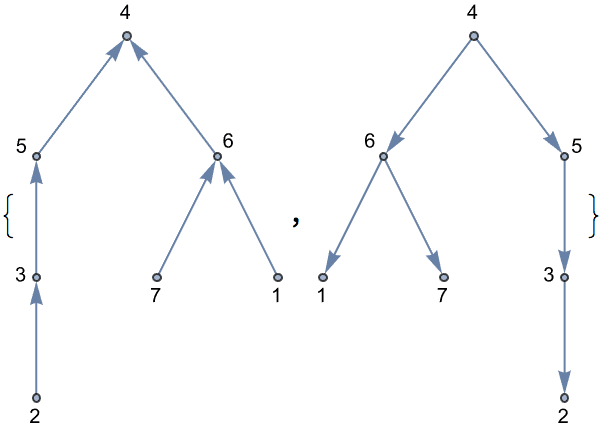
?IGTakeSubgraph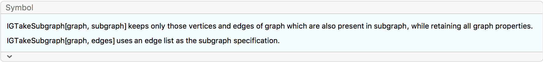
IGTakeSubgraph[graph, subgraph] will effectively
transfer graph properties of a larger graph onto its specified subgraph.
It can be used in conjunction with other graph subsetting functions that
do not retain some or all graph properties, such as
Subgraph, VertexDelete,
NeighborhoodGraph, etc.
If only the edge weights need to be preserved, use
IGWeightedSubgraph when possible. It offers better
performance.
Take a subgraph of a larger graph while preserving all graph properties, including styling attributes.
g = ExampleData[{"NetworkGraph", "EastAfricaEmbassyAttacks"}]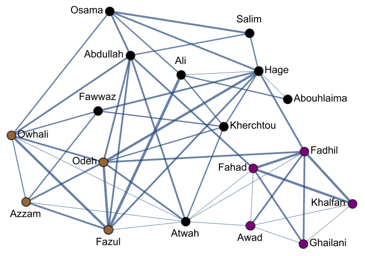
IGTakeSubgraph[g,
Subgraph[
g, {"Osama", "Salim", "Abdullah", "Hage", "Abouhlaima", "Owhali"}]]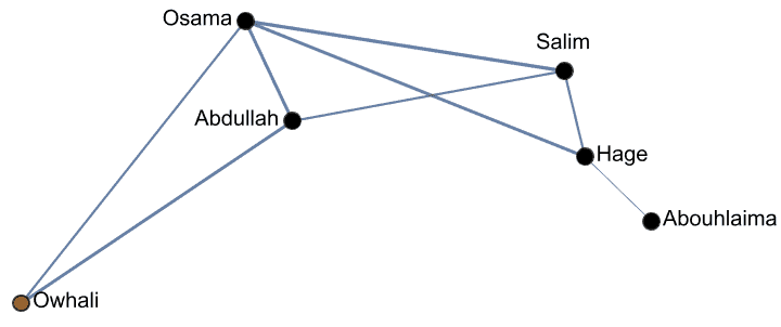
Show the neighbourhood graph of a vertex while preserving vertex shapes.
g = ExampleData[{"NetworkGraph", "SimpleFoodWeb"}]
IGTakeSubgraph[g, NeighborhoodGraph[g, "Sunflower"]]
Take a subgraph of a mesh graph while preserving vertex coordinates.
g = IGMeshGraph[DelaunayMesh@RandomReal[1, {10, 2}],
VertexLabels -> "Name"]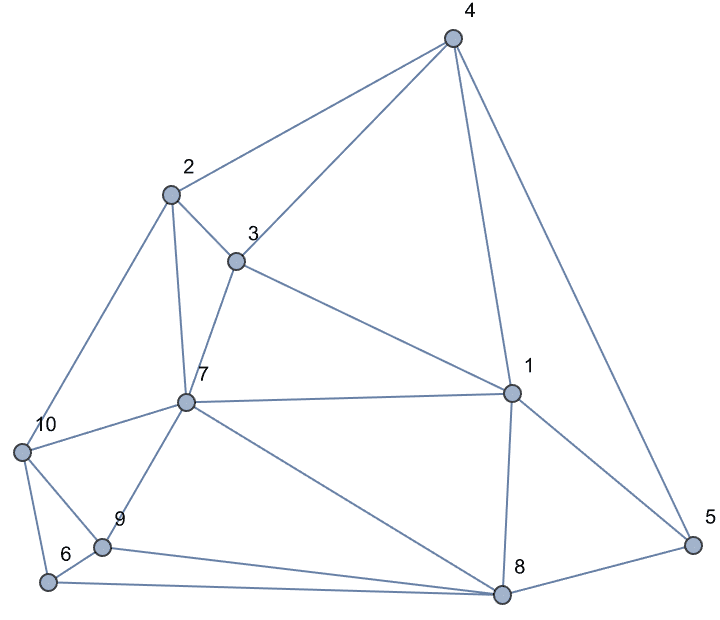
IGTakeSubgraph[g, First@FindHamiltonianCycle[g]]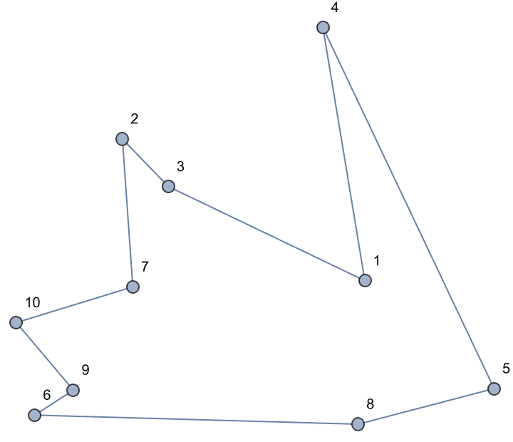
?IGGraphEditor
Experimental: This is experimental functionality that is likely to change significantly in the future.
IGGraphEditor[] typesets an interactive graph editor,
which is convenient for creating small graphs interactively. To add or
remove vertices, or remove edges, click while holding down (Windows
and Linux) or (macOS). To add edges, click the first vertex to
connect, then the second one.
Evaluating the editor using shift-enter creates
a standard Graph object.
Available options:
DirectedEdges -> True creates a directed graph
when no input graph is given.
"KeepVertexCoordinates" -> False will not
preserve the vertex coordinates from the editor view.
"IndexGraph" -> True renumbers vertices using
increasing integers, regardless of their original names in the input
graph.
ImageSize sets the editor size to the given
width.
VertexLabels -> "Name" shows vertex labels in the
editor.
VertexSize sets the vertex size. Valid values are
Tiny, Small, Medium,
Large or a numeric value interpreted as a fraction of the
editor view diagonal.
"PerformanceLimit" sets the maximum number of graph
elements (vertices and edges) that are allowed in the editor. The
default is 450.
"SnapToGrid" -> True will snap vertices to points
on a grid while dragging.
"CreateVertexSelects" -> False disables
immediately selecting newly created vertices to add a
connection.
The editor can be used to modify an existing graph:
IGGraphEditor[CycleGraph[5], VertexLabels -> "Name"]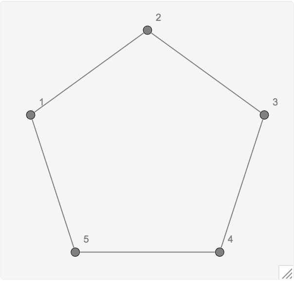
?IGIndexEdgeList
IGIndexEdgeList is useful for implementing graph
processing functions in Mathematica, and is used internally by
many IGraph/M functions that do not call the igraph library.
IGIndexEdgeList[
Graph[{a, b, c}, {b <-> c, c <-> a}]]{{2, 3}, {1, 3}}
Developer`PackedArrayQ[%]True
IGIndexEdgeList[g] is faster than
EdgeList[g] and usually much faster than
EdgeList@IndexGraph[g].
g = ExampleData[{"NetworkGraph", "CondensedMatterCollaborations"}];{First@RepeatedTiming@EdgeList[g],
First@RepeatedTiming@EdgeList@IndexGraph[g],
First@RepeatedTiming@IGIndexEdgeList[g]}{0.00956538, 0.335105, 0.0015711}
List @@@ Sort /@ EdgeList@IndexGraph[g] === Sort /@ IGIndexEdgeList[g]True
A graph can be directly re-built from an index-based edge list.
Graph[{a, b, c}, {{2, 3}, {1, 3}}]![]()
?IGSameGraphQ
IGSameGraphQ checks if two graphs have the same vertex
and edge set. Edge and vertex properties, as well as edge tags, are
ignored.
IGSameGraphQ[IGShorthand["1-2-1", MultiEdges -> True],
Graph[{1 <-> 2, 1 <-> 2}]]True
The vertex names must be the same in order for
IGSameGraphQ to return True.
IGSameGraphQ[IGShorthand["A-B-A", MultiEdges -> True],
Graph[{1 <-> 2, 1 <-> 2}]]False
The order of the edge and vertex lists does not matter.
IGSameGraphQ[Graph[{1 <-> 2, 3 <-> 4}],
Graph[{4 <-> 3, 1 <-> 2}]]True
For non-Graph expressions, IGSameGraphQ
returns False.
IGSameGraphQ[1, 2]False
?IGCanonicalLabeledGraph
IGCanonicalLabeledGraph creates a canonical version of
labelled graphs so that
IGCanonicalLabeledGraph[g1] === IGCanonicalLabeledGraph[g2]
holds precisely when IGSameGraphQ[g1, g2].
This function discards all graph properties, as well as edge tags.
g1 = Graph[{4 <-> 3, 1 <-> 2},
VertexLabels -> Automatic];
g2 = Graph[{1 <-> 2, 3 <-> 4},
VertexLabels -> Automatic];
IGCanonicalLabeledGraph[g1] === IGCanonicalLabeledGraph[g1]True
IGCanonicalLabeledGraph is useful in conjunction with DeleteDuplicatesBy.
DeleteDuplicatesBy[{g1, g2, g1}, IGCanonicalLabeledGraph]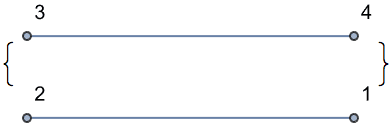
?IGCanonicalEdgeList
IGCanonicalEdgeList canonicalizes an edge list in a way
similar to IGCanonicalLabeledGraph.
IGSameGraphQ[g1, g2] is equivalent to
IGCanonicalEdgeList@EdgeList[g1] === IGCanonicalEdgeList@EdgeList[g2]
when g1 and g2 have no isolated vertices.
This function discards edge tags.
IGCanonicalLabeledEdgeList is useful in conjunction with
DeleteDuplicatesBy.
Highlight all distinct \(K_{3,3}\) subgraphs of a Queen graph:
g = GraphData[{"Queen", {2, 4}}];
sg = CompleteGraph[{3, 3}];HighlightGraph[g, Graph[#], GraphHighlightStyle -> "Thick"] & /@
DeleteDuplicatesBy[
IGCanonicalEdgeList@EdgeList[sg] /.
IGLADFindSubisomorphisms[sg, g],
IGCanonicalEdgeList
]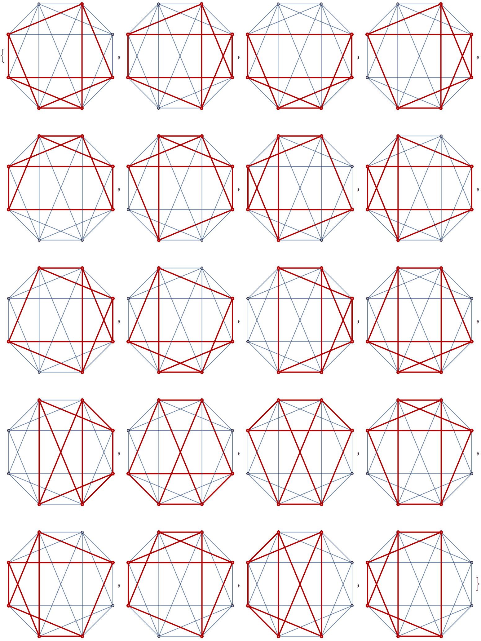
?IGAdjacentVerticesQ
IGAdjacentVerticesQ[graph, {u, v}] tests if there is an
edge from u to v.
g = CycleGraph[6, DirectedEdges -> True, VertexLabels -> "Name"]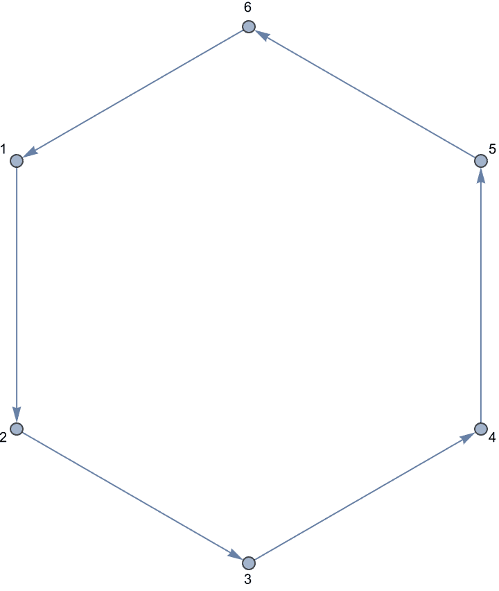
IGAdjacentVerticesQ[g, {1, 2}]True
Edge directions are taken into account:
IGAdjacentVerticesQ[g, {2, 1}]False
The following vertices are not adjacent:
IGAdjacentVerticesQ[g, {1, 3}]False
Vertices that are not part of the graph are allowed. They are considered not to be adjacent:
IGAdjacentVerticesQ[g, {"x", 2}]False
?IGPartitionsToMembership
?IGMembershipToPartitions
A partitioning of a set of elements can be represented in multiple ways. One way is to list the members of each partition. Another is to annotate each element with the index of the partition it belongs to, i.e. construct a “membership vector”. These functions convert between these representations.
IGraph/M generally uses disjoint subsets to represents partitions. Membership vectors are useful when storing the membership information as vertex attributes, or when exchanging data with other interfaces of igraph.
IGPartitionsToMembership[{a, b, c, d}, {{a, c}, {d, b}}]{1, 2, 1, 2}
IGMembershipToPartitions[{a, b, c, d}, {1, 2, 1, 2}]{{a, c}, {b, d}}
If the given partitions do not cover the element set, the missing
elements will be marked with 0 in the membership
vector.
IGPartitionsToMembership[{a, b, c, d}, {{a}, {b, d}}]{1, 2, 0, 2}
The following graph has the type of nodes encoded as a vertex attribute.
g = ExampleData[{"NetworkGraph", "BipartiteDiseasomeNetwork"}];
IGVertexProp["Type"][g] // Short![]()
Let us extract the attribute values as a vector and construct the two vertex partitions.
parts = IGMembershipToPartitions[g, IGVertexProp["Type"][g]];Verify that the graph is bipartite according to this partitioning.
IGBipartiteQ[g, parts]True
Annotate the vertices of a bipartite graph with their computed membership value.
g = IGBipartiteGameGNM[5, 6, 14, VertexSize -> Large];g = IGVertexMap[
# &,
"membership" ->
IGPartitionsToMembership[VertexList[g]]@*IGBipartitePartitions,
g
];Colour the vertices accordingly.
IGVertexMap[ColorData[100], VertexStyle -> IGVertexProp["membership"],
g]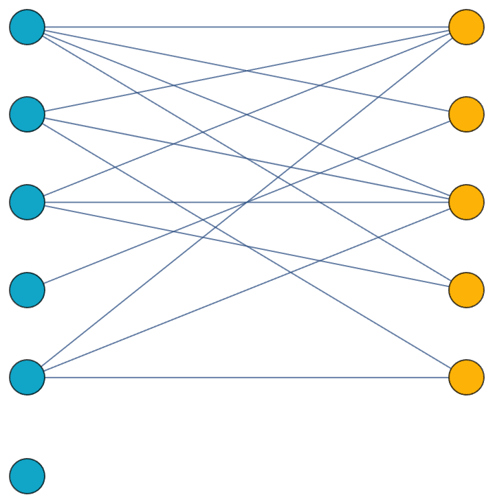
Visualize a vertex colouring using HighlightGraph.
g = IGSquareLattice[{2, 2, 2, 2}, "Periodic" -> True]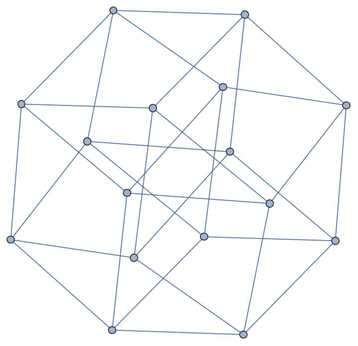
HighlightGraph[
g, IGMembershipToPartitions[g, IGVertexColoring[g]],
VertexSize -> Medium, GraphHighlightStyle -> "DehighlightGray"
]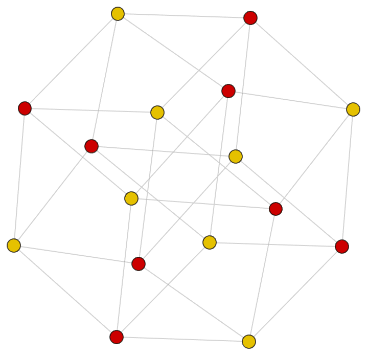
?IGReorderVertices
IGReorderVertices changes the order in which graph
vertices are stored. The graph itself is not modified, only its
representation. The ordering of vertices affects how several of
Mathematica’s graph processing functions work.
Let us use a styled graph for illustration, to demonstrate that graph properties are preserved.
g1 = RandomGraph[{5, 5},
VertexStyle -> {1 -> LightRed, 3 -> LightGreen},
VertexSize -> Medium, VertexLabels -> Placed[Automatic, Center]]
g2 = IGReorderVertices[{5, 4, 3, 2, 1}, g1]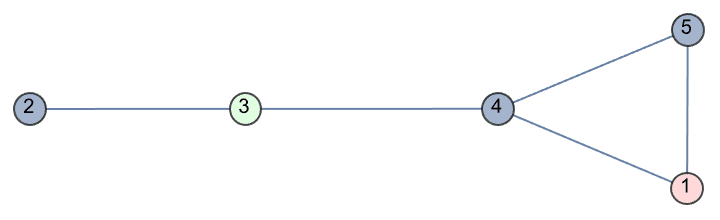
VertexList /@ {g1, g2}{{1, 2, 3, 4, 5}, {5, 4, 3, 2, 1}}
IGIsomorphicQ[g1, g2]True
The result of certain operations, such as
DirectedGraph[…, "Acyclic"] or
AdjacencyMatrix, depends on the vertex ordering.
DirectedGraph[#, "Acyclic"] & /@ {g1, g2}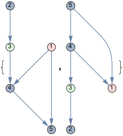
Order the vertices of a directed acyclic graph so that its adjacency matrix is upper triangular.
g = RandomGraph[{10, 30}, DirectedEdges -> True];
g = EdgeDelete[g, IGFeedbackArcSet[g]];
ArrayPlot /@
AdjacencyMatrix /@ {g, IGReorderVertices[TopologicalSort[g], g]}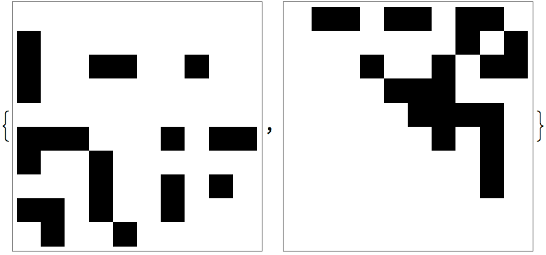
Visualize a graph so that a Hamiltonian cycle is on a circle.
g = GraphData["DodecahedralGraph"];
IGLayoutCircle@
IGReorderVertices[FindHamiltonianCycle[g][[1, All, 1]], g]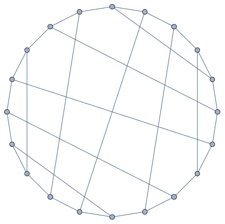
Change the order how graph vertices are drawn in a circular layout without discarding any styling or other properties.
g = IGLayoutCircle[
ExampleData[{"NetworkGraph", "EastAfricaEmbassyAttacks"}],
VertexLabels -> (_ -> Placed["Name", Tooltip])
]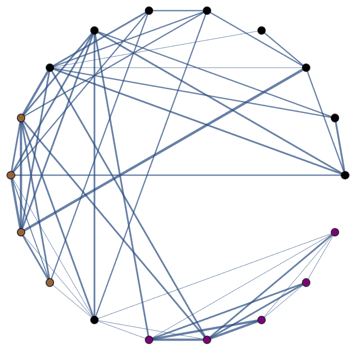
IGLayoutCircle@IGReorderVertices[RandomSample@VertexList[g], g]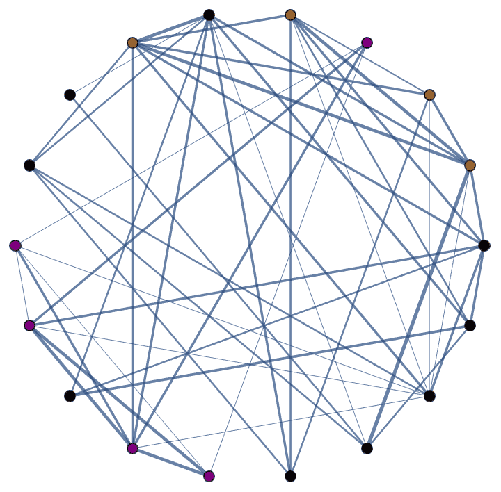
Reorder the vertices of a bipartite graph to make the bipartite
structure explicit in its adjacency matrix. Note that if the goal is
simply visualizing the adjacency matrix,
IGAdjacencyMatrixPlot can be used instead.
g = CycleGraph[10];
ArrayPlot /@
AdjacencyMatrix /@ {g,
IGReorderVertices[Flatten@IGBipartitePartitions[g], g]}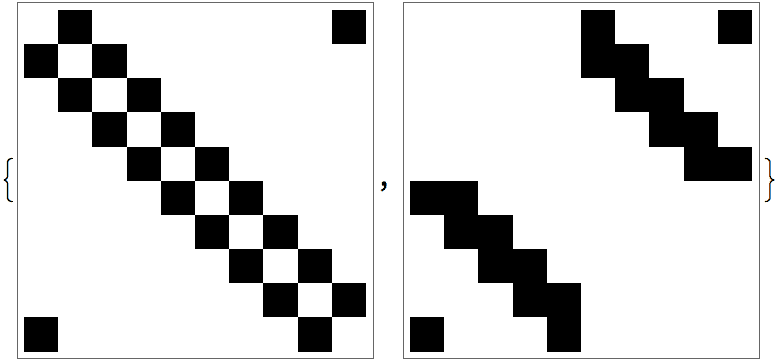
Order the vertices of a graph by increasing degree.
g = RandomGraph[{20, 40}];
{IGLayoutCircle[g],
IGLayoutCircle@
IGReorderVertices[VertexList[g][[Ordering@VertexDegree[g]]], g]}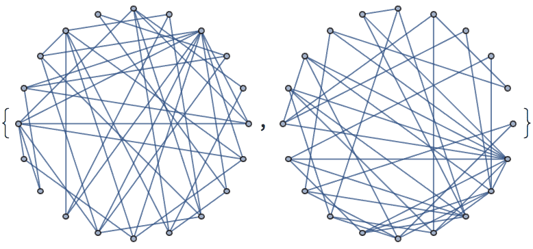
?IGAdjacencyList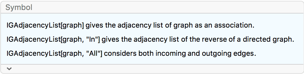
IGAdjacencyList returns the adjacency list of a graph as
an association. This is often a more useful format than what the
built-in AdjacencyList provides.
IGAdjacencyList[Graph[{1 <-> 2}]]<|1 -> {2}, 2 -> {1}|>
For directed graphs, only outgoing edges are considered when building
the adjacency list. In contrast, the built-in AdjacencyList
ignores edge directions.
IGAdjacencyList[Graph[{1 -> 2}]]<|1 -> {2}, 2 -> {}|>
AdjacencyList[Graph[{1 -> 2}]]{{2}, {1}}
Consider incoming edges instead.
IGAdjacencyList[Graph[{1 -> 2}], "In"]<|1 -> {}, 2 -> {1}|>
Consider both incoming and outgoing edges.
IGAdjacencyList[Graph[{1 -> 2}], "All"]<|1 -> {2}, 2 -> {1}|>
With this option, reciprocal edges are considered individually in directed graphs.
IGAdjacencyList[Graph[{1 -> 2, 2 -> 1}], "All"]<|1 -> {2, 2}, 2 -> {1, 1}|>
Multi-edges and self-loops are supported. In contrast, the built-in
AdjacencyList ignores them.
IGAdjacencyList[Graph[{1 -> 2, 1 -> 2, 2 -> 2, 2 -> 2}]]<|1 -> {2, 2}, 2 -> {2, 2}|>
AdjacencyList[Graph[{1 -> 2, 1 -> 2, 2 -> 2}]]{{2}, {1, 2}}
Self-loops are traversed in only one direction in undirected graphs.
Thus the result of the below is not
<|1 -> {1, 1}|> but simply
<|1 -> {1}|>. This is consistent with
AdjacencyMatrix, but not with
VertexDegree.
IGAdjacencyList[Graph[{1 <-> 1}]]<|1 -> {1}|>
IGAdjacencyList can be used to find the parent of each
node in a rooted tree. The root itself will have no parent.
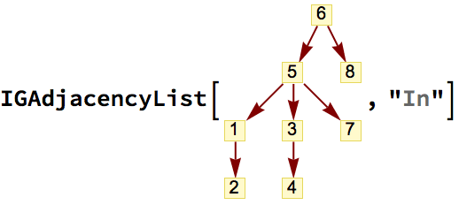
<|1 -> {5}, 2 -> {1}, 3 -> {5}, 4 -> {3}, 5 -> {6}, 6 -> {}, 7 -> {5}, 8 -> {6}|>
Find the children of each node.
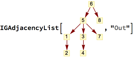
<|1 -> {2}, 2 -> {}, 3 -> {4}, 4 -> {}, 5 -> {1, 3, 7}, 6 -> {5, 8}, 7 -> {}, 8 -> {}|>
?IGAdjacencyGraph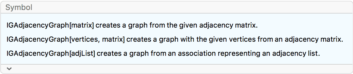
IGAdjacencyGraph can convert an adjacency matrix or an
adjacency list representation of a graph into a Graph
expression. When given a matrix, it behaves equivalently to the built-in
function AdjacencyGraph.
The available options are:
DirectedEdges -> True and
DirectedEdges -> False create a directed or undirected
graph, respectively. The default setting is
DirectedEdges -> Automatic, which creates an undirected
graph when this is consistent with the given adjacency matrix or
adjacency list.Compute the adjacency list of a graph, then convert it back to a
Graph expression.
g = RandomGraph[{5, 6}, DirectedEdges -> True, VertexLabels -> "Name"]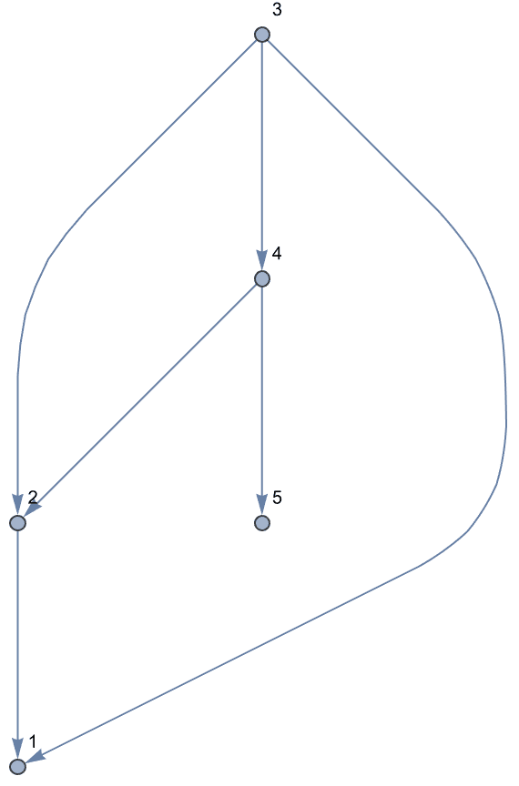
IGAdjacencyList[g]<|1 -> {}, 2 -> {1}, 3 -> {1, 2, 4}, 4 -> {2, 5}, 5 -> {}|>
IGAdjacencyGraph[%]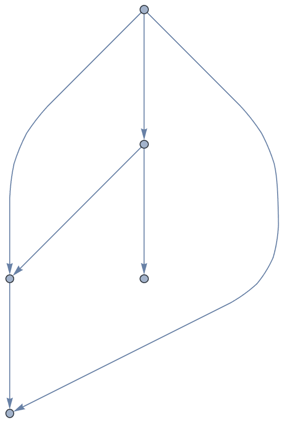
The representation of combinatorial embeddings used by IGraph/M is also a valid adjacency list.
IGPlanarEmbedding@CompleteGraph[4]<|1 -> {2, 3, 4}, 2 -> {1, 4, 3}, 3 -> {2, 4, 1}, 4 -> {3, 2, 1}|>
IGAdjacencyGraph[%]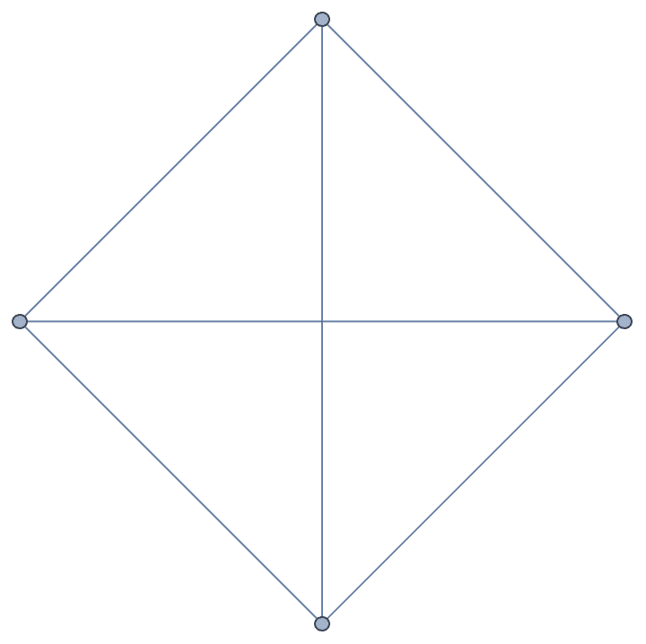
?IGVertexAssociate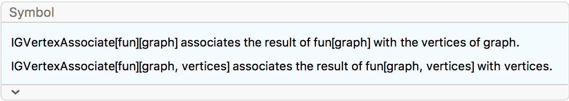
IGVertexAssociate[fun] is an operator that, when applied
to graph, will associate the result of
fun[graph] with each vertex.
In Mathematica, functions that compute a value for each
vertex always return a list, with the values ordered to correspond to
the VertexList of the graph. In many situations, it is more
convenient to use an association where the keys are the vertex names. If
fun is a function that computes a vertex property and gives
the result as a list, the operator IGVertexAssociation[fun]
will give an association instead.
Get the betweenness of a vertex by name:
net = ExampleData[{"NetworkGraph", "Friendship"}]
betw = IGVertexAssociate[IGBetweenness][net]<|"Anna" -> 15.5, "Rose" -> 0.5, "Nora" -> 1., "Ben" -> 0.5, "Larry" -> 5.5, "Carol" -> 0., "Rudy" -> 4.5, "Linda" -> 1.5, "James" -> 1.|>
betw["Larry"]5.5
IGraph/M has many functions which can be restricted to compute values
for only a subset of vertices. These use the syntax
fun[graph, vertices]. If fun supports this
syntax, then IGVertexAssociate[fun] also takes a vertex
list as its second argument.
IGVertexAssociate[IGEccentricity][net, {"Anna", "James", "Rudy"}]<|"Anna" -> 2, "James" -> 3, "Rudy" -> 2|>
Smoothen away the degree-2 vertices of a graph while retaining the coordinates of each vertex:
g = IGGiantComponent@RandomGraph[{100, 100}]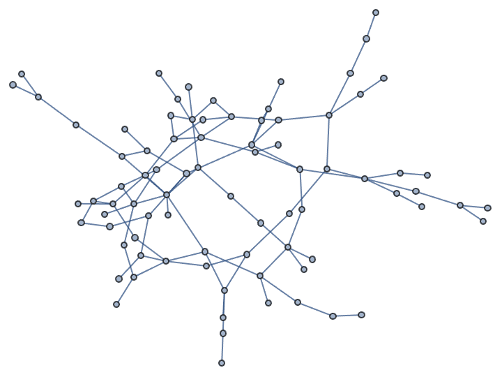
g2 = IGSmoothen[g] //
IGVertexMap[IGVertexAssociate[GraphEmbedding][g],
VertexCoordinates -> VertexList]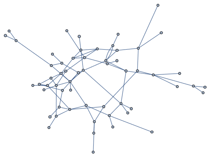
Compare the smoothened graph with the original in a flip view:
FlipView[{g, g2}]
Extract a vertex property as an association:
IGVertexAssociate[IGVertexProp["Group"]]@
ExampleData[{"NetworkGraph", "EastAfricaEmbassyAttacks"}]<|"Osama" -> "Planners", "Salim" -> "Planners", "Ali" -> "Planners", "Abouhlaima" -> "Planners", "Kherchtou" -> "Planners", "Fawwaz" -> "Planners", "Abdullah" -> "Planners", "Hage" -> "Planners", "Odeh" -> "Nairobi Cell", "Owhali" -> "Nairobi Cell", "Fazul" -> "Nairobi Cell", "Azzam" -> "Nairobi Cell", "Atwah" -> "Planners", "Fahad" -> "Dar es Salaam Cell", "Fadhil" -> "Dar es Salaam Cell", "Khalfan" -> "Dar es Salaam Cell", "Ghailani" -> "Dar es Salaam Cell", "Awad" -> "Dar es Salaam Cell"|>
?IGTryUntil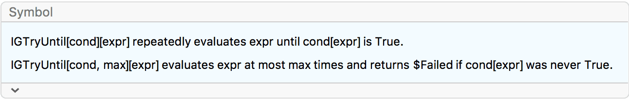
IGTryUntil repeatedly evaluates an expression until the
result of the evaluation satisfies a condition. It is particularly
useful for concisely implementing rejection sampling.
Choose 10 distinct random primes not greater than 100:
IGTryUntil[DuplicateFreeQ][RandomPrime[100, 10]]{53, 61, 73, 41, 43, 19, 17, 67, 37, 11}
Create a power-law distributed degree sequence and build a corresponding graph:
IGRealizeDegreeSequence[
IGTryUntil[IGGraphicalQ]@RandomVariate[ZipfDistribution[1], 100]
]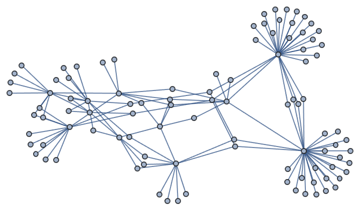
Generate a random tree (a connected graph) with a given degree sequence using the configuration model:
ds = {3, 3, 3, 3, 3, 3, 2, 2, 2, 2, 2, 2, 1, 1, 1, 1, 1, 1, 1, 1};
IGTryUntil[IGConnectedQ]@
IGDegreeSequenceGame[ds, Method -> "ConfigurationModelSimple"]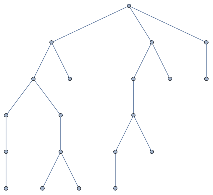
Some result will occur very infrequently or not at all, so it is
useful to limit the number of trials. The following attempts to generate
a random non-connected cubic graph on 50 vertices, and simply returns
$Failed if it does not succeed after 100 tries.
IGTryUntil[Not@*IGConnectedQ, 100][
IGDegreeSequenceGame[
ConstantArray[3, 50],
Method -> "ConfigurationModelSimple"
]
]$Failed
The IGData[] function provides access to various useful
datasets. In particular, it can list small directed graphs ordered based
on their IGIsoclass[], i.e. the same order that motif
counting functions use.
?IGData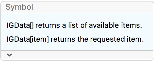
List the available datasets:
IGData[]{{"AllDirectedGraphs", 2}, {"AllDirectedGraphs", 3}, {"AllDirectedGraphs", 4}, {"AllUndirectedGraphs", 2}, {"AllUndirectedGraphs", 3}, {"AllUndirectedGraphs", 4}, {"AllUndirectedGraphs", 5}, {"AllUndirectedGraphs", 6}, "MANTriadLabels"}
These are all size 3 directed graphs:
IGData[{"AllDirectedGraphs", 3}] //
Map[Framed@
Labeled[Graph[#, ImageSize -> 50],
IGIsoclass[#]] &] // Multicolumn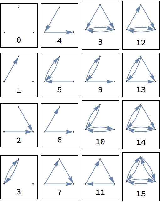
"MANTriadLabels" refers to the mutual, asymmetric, null
labelling of triads used by IGTriadCensus[]. Each label is
mapped to the corresponding graph, ordered based on their
IGIsoclass. This is useful for converting the output of
IGTriadCensus[] to a format compatible with
IGMotifs[].
g = RandomGraph[{20, 50}, DirectedEdges -> True];
{IGMotifs[g, 3],
Lookup[IGTriadCensus[g], Keys@IGData["MANTriadLabels"]]} // Grid![]()
The IGGraphAtlas function provides access to the graphs
listed in An Atlas of Graphs by Ronald C. Read and Robin J. Wilson,
Oxford University Press, 1998.
?IGGraphAtlas
IGGraphAtlas[341]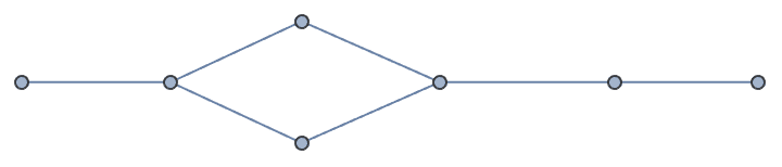
Finally, remember that Mathematica itself comes with a large database of graphs and their properties, accessible through GraphData.
The IGLatticeMesh function includes a set of pre-defined
two-dimensional lattice structures. Evaluate
IGLatticeMesh[] to get the list of available lattices.
The data used by IGMeshGraph was sourced from
Wolfram|Alpha and Mathematica’s curated data system in April
2018.
?IGLatticeMesh
IGLatticeMesh[]{"Square", "Hexagonal", "Triangular", "Trihexagonal", \ "SmallRhombitrihexagonal", "TruncatedSquare", "SnubSquare", \ "TruncatedHexagonal", "ElongatedTriangular", \ "GreatRhombitrihexagonal", "SnubHexagonal", "Rhombille", \ "DeltoidalTrihexagonal", "TetrakisSquare", "CairoPentagonal", \ "TriakisTriangular", "PrismaticPentagonal", "BisectedHexagonal", \ "FloretPentagonal", "DellaRobbiaWeave", "Portugal", "StackBond", \ "Herringbone", "Basketweave", "PersianHexagonalWeave", "Hopscotch", \ "StretcherBond", "Pinwheel", "BrickworkSquare", "Chickenwire", \ "Corridor", "CorridorHorizontal", "Brickweave", "Trellis", \ "HeeschIsohedral", "PPentomino", "Chevron", "Shingle", "Zigzag", \ "Kite", "FalseCubic", "TrihexAndHex", "GlideReflection", \ "PentagonType1", "PentagonType2", "PentagonType3", "PentagonType4", \ "PentagonType5", "PentagonType6", "PentagonType7", "PentagonType8", \ "PentagonType9", "PentagonType10", "PentagonType11", \ "PentagonType12", "PentagonType13", "PentagonType14", \ "PentagonType15"}
IGraph/M makes use of Mathematica’s own random number
generator by default, thus functions like SeedRandom and
BlockRandom have the expected effect.
SeedRandom[137];
Table[BlockRandom@IGErdosRenyiGameGNM[6, 9], {3}]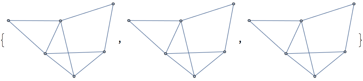
BlockRandom is useful for example to get consistent
graph layouts without affecting subsequent uses of the random number
generator.
g = RandomGraph[{100, 150}];
Table[IGLayoutFruchtermanReingold[g], {4}]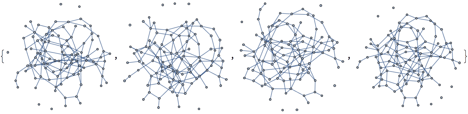
Table[BlockRandom[SeedRandom[1234];
IGLayoutFruchtermanReingold[g]], {4}]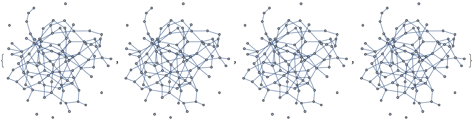
IGraph/M can be configured to either use Mathematica’s
built-in generator, or the default generator of the igraph C library.
The default generator of igraph will perform better, but it does not
react to BlockRandom and must be seeded with
IGSeedRandom (not with SeedRandom).
Benchmark IGRandomWalk when using Mathematica’s
random number generator:
g = IGGiantComponent@RandomGraph[{1000, 2000}];IGRandomWalk[g, 1, 10000000]; // RepeatedTiming{0.598208, Null}
Benchmark it with igraph’s default generator:
IGSeedRandom[Method -> "igraph"]
IGRandomWalk[g, 1, 10000000]; // RepeatedTiming{0.366929, Null}
Set the generator back to Mathematica’s:
IGSeedRandom[Method -> "Mathematica"]?IGSeedRandom
Available Method option values are:
"Mathematica" uses Mathematica’s built-in random
number generator. With this choice, functions like
SeedRandom and BlockRandom will IGraph/M
functions as expected. Performance is not as good as with the
"igraph" generator
"igraph" uses the core igraph C library’s random
number generator. SeedRandom and BlockRandom
have no effect on this generator. Seeding can be done with
IGSeedRandom. Performance is better than with the
"Mathematica" generator.
Experimental: This is experimental functionality that may change in the future.
Some igraph functions can report their progress while working. IGraph/M contains experimental functionality that exposes igraph’s progress reports. This functionality may change without notice in the future.
?IGraphM`Progress`*
Show the progress indicator.
IGraphM`Progress`Indicator[]![]()
Progress reporting has a performance cost, therefore it is disabled by default. To enable it, use:
IGraphM`Progress`SetReporting[True]When a computation that supports progress reporting is running, the indicator will show the status.
compute[] :=
IGCommunitiesGreedy@
IGStochasticBlockModelGame[0.02 IdentityMatrix[10] + 0.005,
ConstantArray[800, 10]];
compute[];By default, the progress indicator is updated only if progress has increased by at least 1%. In other words, the reporting granularity is 1%. The lower the granularity value, the higher the performance impact of reporting.
Change the reporting granularity to 10%.
IGraphM`Progress`SetReporting[True, "Granularity" -> 10]Follow the progress by dynamically showing the value of internal progress variables:
Dynamic@{IGraphM`Progress`Message, IGraphM`Progress`Percent}
compute[];![]()
Disable progress reporting and set the granularity to its default values (in case it gets enabled again later).
IGraphM`Progress`SetReporting[False, "Granularity" -> Automatic]The following symbols and functions can be used to retrieve the IGraph/M version.
?IGVersion
IGVersion[]"IGraph/M 0.6.5 (December 21, 2022) igraph 0.9.10-23-g5635203bd (Dec 21 2022) Mac OS X x86 (64-bit)"
?IGraphM`Information`$Version
IGraphM`Information`$Version"0.6.5 (December 21, 2022)"
If you need help with using this package, the following support options are available:
Post on the igraph
discussion forum and tag the post as
Mathematica.
Post on the Mathematica
StackExchange and tag the post as igraphm.
If you find a problem with IGraph/M or its documentation, please
report it through the GitHub issue
tracker or the igraph
discussion forum. Always include the output of the
GetInfo[] function with problem reports.
?IGraphM`Developer`GetInfo
Most functions in IGraph/M are based on the igraph C library, originally written by Gábor Csárdi and Tamás Nepusz. To cite the igraph C library in publications, see “Citing igraph” in the igraph Reference Manual. Website: https://igraph.org/
Some functions, in particular in the area of planar graphs, use the LEMON graph library. Website: https://lemon.cs.elte.hu/
Some proximity graph functions make use of the nanoflann library. Website: https://github.com/jlblancoc/nanoflann
IGraph/M was developed with the Wolfram Language Plugin for IntelliJ IDEA by Patrick Scheibe. Without the help of this IDE, it would have been difficult to manage the complexity of this package. Website: http://wlplugin.halirutan.de/
The web version of the documentation is prepared with the M2MD package by Kuba Podkalicki. Website: https://github.com/kubaPod/M2MD/
The help of the Mathematica StackExchange community was invaluable while developing this package.
People who have contributed to IGraph/M:
Szabolcs Horvát (main author and maintainer)
Henrik Schumacher (help with mesh-graph conversion and proximity graph functions)
Juho Lauri (advice with the implementation of graph colouring functions)
Kuba Podkalicki (implementation of
IGGraphEditor[])
To cite IGraph/M in a publication, please refer to:
Sz. Horvát, J. Podkalicki, G. Csárdi, T. Nepusz, V. Traag, F. Zanini, D. Noom, IGraph/M: graph theory and network analysis for Mathematica, preprint (2022), doi:10.48550/arXiv.2209.09145
IGraphM/ on Zenodo, doi:10.5281/zenodo.1134932
Copyright © 2016-2022 Szabolcs Horvát
This program is free software: you can redistribute it and/or modify it under the terms of the GNU General Public License as published by the Free Software Foundation, either version 3 of the License, or (at your option) any later version.
This program is distributed in the hope that it will be useful, but WITHOUT ANY WARRANTY; without even the implied warranty of MERCHANTABILITY or FITNESS FOR A PARTICULAR PURPOSE. See the GNU General Public License for more details.
You should have received a copy of the GNU General Public License along with this program. If not, see https://www.gnu.org/licenses/