Quiz Solution
PHYS205 Electricity and Magnetism
We shall assume that the magnetic field  and the angular velocity vector
  point in the same direction (
 ⋅
⋅ > 0). The Lorentz force causes the positive
charges to move outward in the sphere, so a negative space charge will build up in
the interior, while the surface charge will be positive.
> 0). The Lorentz force causes the positive
charges to move outward in the sphere, so a negative space charge will build up in
the interior, while the surface charge will be positive.
The charges distribute themselves in such a way that the electric field balances
the Lorentz force. The sphere is not a perfect conductor, so in a steady state the
charges must move with exactly the same velocity  =
=  ×
× as the sphere at
every point. (To keep the charges in motion relative to the sphere an
electromotive force would be necessary.)
as the sphere at
every point. (To keep the charges in motion relative to the sphere an
electromotive force would be necessary.)
 | (1) |
The space charge density ρ can be found by taking the divergence of this
equation.
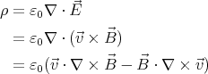 | (2) |
Here we used the fact that a mixed product does not change when its terms are
cyclically permuted:  ⋅ (
⋅ ( ×
× ) =
) =  ⋅ (
⋅ ( ×
× ). According to Maxwell’s equations
∇×
). According to Maxwell’s equations
∇× = μ0
= μ0 = μ0ρ
= μ0ρ .
.

Substituting these results back into equation (2), ρ = ε0μ0v2ρ - 2ε
0 ⋅
⋅ . Using
the formula ε0μ0 = 1∕c2 we get
. Using
the formula ε0μ0 = 1∕c2 we get
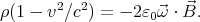 | (3) |
Since v ≪ c, 1 - v2∕c2 ≈ 1. To use equation (3) to get the space charge density,
the magnetic field  needs to be known. But the homogeneous magnetic
field will be distorted by the field originating from the circulating charges
in the sphere. If the sphere is not spinning very fast, this correction is
relatively small and the following method can be used to approximate
needs to be known. But the homogeneous magnetic
field will be distorted by the field originating from the circulating charges
in the sphere. If the sphere is not spinning very fast, this correction is
relatively small and the following method can be used to approximate
 :
:
First we assume that the applied homogeneous magnetic field is unchanged
and denote it by  0, then calculate the space charge ρ and current densities
 = ρ
= ρ . Next, we use these currents to find the correction
  1 to the homogeneous
field, and find the corrected charge densities and currents using
1 to the homogeneous
field, and find the corrected charge densities and currents using  0 +
0 +  1. With
these new current densities the next correction
1. With
these new current densities the next correction  2 can be calculated. The result
can be made more accurate by doing more iterations.
2 can be calculated. The result
can be made more accurate by doing more iterations.
Without carrying out the actual calculations, we know that B1 ~ μ0I∕R,
where I is a current-like quantity: I ~ ωRρR2. But ρ ~ ε
0ωB0, so
B1 ~ μ0ε0ω2R2B
0 = v2∕c2B
0. Thus, when using the v ≪ c approximation, the
corrections to the homogeneous field due to the induced rotating space charge can
be neglected. Further on,  shall be considered homogeneous.
Now we proceed with calculating the electric field and potential inside the
sphere. Substituting  =
=  ×
× into equation (1) we get
  = -
= - (
( ⋅
⋅ ) +
) +  (
( ⋅
⋅ ).
).
 and
and  are parallel, so
  = -
= - (
( ⋅
⋅ ), where a is the distance from the axis of
rotation: if we choose ẑ∥
), where a is the distance from the axis of
rotation: if we choose ẑ∥ , then
  = x
= x + yŷ.
+ yŷ.
It must be noted here that the electric field can compensate the Lorentz force
only if ∇× ( ×
× ) = 0. This is true for a homogeneous
  -field approximation
when the axis of rotation is parallel to the magnetic field, but not otherwise. If the
Lorentz force can not be completely cancelled, there will always be some charge
motion relative to the sphere until the energy dissipation causes the spinning
sphere to stop.
-field approximation
when the axis of rotation is parallel to the magnetic field, but not otherwise. If the
Lorentz force can not be completely cancelled, there will always be some charge
motion relative to the sphere until the energy dissipation causes the spinning
sphere to stop.
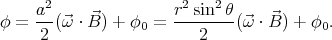
The electric potential inside the sphere is
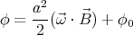
In spherical coordinates ϕ = ϕ0 -r2 sin 2θ ( ⋅
⋅ )∕2, where θ is the angle between
 and the axis of rotation. Unlike
  , the potential is continuous over the surface of
the sphere, so the boundary condition ϕ = ϕ0 -R2 sin 2θ (
, the potential is continuous over the surface of
the sphere, so the boundary condition ϕ = ϕ0 -R2 sin 2θ ( ⋅
⋅ )∕2 may be used to
also find ϕ outside the sphere of radius R.
)∕2 may be used to
also find ϕ outside the sphere of radius R.
Let us approximate a potential that satisfies this boundary condition with
multipole terms! The monopole term must be zero because the total charge of the
sphere is zero. The dipole term is also zero because the dipole field does not
match the symmetry of this system. Therefore the dominant part of the sought
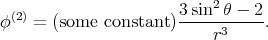
potential must be a quadrupole potential. It is easy to see that the potential ϕ(2)
of a quadrupole that was created by superposing two dipoles along their axes (to
satisfy the requirement of azimuthal symmetry) satisfies the boundary conditions
exactly:
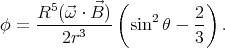
We need to seek no further: outside the sphere the potential will be
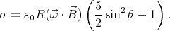
The surface charge density is σ =  r=R.
r=R.
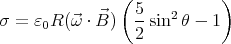
By integrating this over the surface of the sphere we see that indeed the total
surface charge equals the total volume charge in magnitude, so the sphere has no
net charge.
Summary
The potential inside the sphere is
The electric field inside the sphere is
 | = - ( ( ⋅ ⋅ ) ) | |
|
| Er | = -r sin 2θ ( ⋅ ⋅ ) ) | |
|
| Eθ | = -r sin θ cos θ ( ⋅ ⋅ ). ). | | |
The potential outside the sphere is
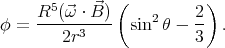
The electric field outside the sphere is
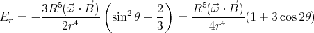
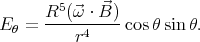
The surface charge density is