It can be proven that this is the only solution using an argument similar
to that found in Griffiths’ book (page 118, second uniqueness theorem),
but using the displacement vector  instead of
  .
.
If the sphere is pushed “deeper” into the dielectric (fig. 2a), the potential cannot stay unchanged because the electric field will no longer be parallel to the surface of the dielectric and bound charges will be induced. In the case illustrated on fig. 2b, the potential will not change.
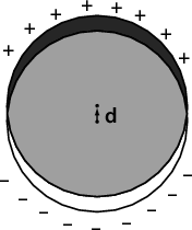
If the total charge of the sphere is constant, the charges will redistribute on the surface of the sphere in such a way that the electric field can stay spherically symmetric. On the lower hemisphere the bound charges will reduce the total (bound + free) surface charge density by a factor of ε. Thus, if the total free charge is Qfree, and the total charge is Q, Q∕2 + εQ∕2 = Qfree ⇒ Q = 2Qfree∕(1 + ε). The potential will be reduced by a factor of 2∕(1 + ε) everywhere in space.
 0.
0.
The polarization of the dielectric is  0 = ε0χ
 0 where χ = εr -1 is the
susceptibility of the material. We shall need to consider regions with
uniform polarization -
0 where χ = εr -1 is the
susceptibility of the material. We shall need to consider regions with
uniform polarization - 0.
0.
- Spherical region
What is the electric field inside a uniformly polarized sphere, of polarization
 ?
?
A uniformly polarized sphere can be imagined as two superposed uniformly but oppositely charged spheres, slightly displaced by
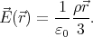
 . The electric field inside a uniformly charged sphere with
charge density ρ, at position
. The electric field inside a uniformly charged sphere with
charge density ρ, at position  relative to the sphere’s centre
is
relative to the sphere’s centre
is
The electric field inside the superposed spheres is
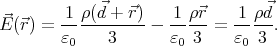
The polarization vector can be thought of as a density of electric dipole moments, so
 = ρ
= ρ , and the electric field inside the polarized
region is
, and the electric field inside the polarized
region is

The electric field in a spherical cavity is
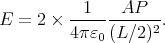
- Needle-shaped region Let us denote the tiny base surface of the
needle with A. Then the bound charges induced by the polarization
will be two point like charges of magnitude AP at the tips of the
needle.
Thus the electric field in the middle of a needle of length L is
The electric field in a cavity is
- Wafer-shaped region A polarized flat region is just like the
capacitor: two parallel sheets of bound charges, with surface
charge density σ = P. The electric field inside this region is just
E = σ∕ε0 = P∕ε0.
Thus the electric field in a thin wafer shaped cavity is

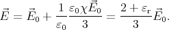
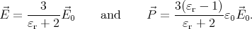
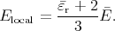
 0? As shown in the previous exercise, the electric field created
by a polarized sphere is
0? As shown in the previous exercise, the electric field created
by a polarized sphere is  inside =
  ∕(3ε0). The total electric field
in the sphere is
∕(3ε0). The total electric field
in the sphere is  =
=  0 -
0 - inside and
  = ε0χ
= ε0χ = ε0(εr - 1)
 ,
so
,
so
The dipole moment of a sphere of volume V and polarization  is
is  = V
= V  ,
so the polarizability of a sphere is α = 3V ε0
,
so the polarizability of a sphere is α = 3V ε0 .
.
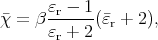
Let us assume that that all the droplets have volume V and there are N droplets per unit volume: NV = β.
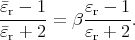
By definition, if  is the susceptibility of the emulsion,
  its polarization,
and
its polarization,
and  the electric field inside, then
  =
= 
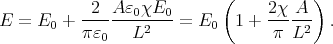
 . If the density of the
droplets is low (β ≪ 1), we can consider the field polarizing a droplet
to be
. If the density of the
droplets is low (β ≪ 1), we can consider the field polarizing a droplet
to be  , so p = α
 and
and  = Np = Nα
 . In this case
  = Nα
and
= Nα
and
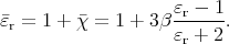
However,  is the average field in the emulsion, and a precise treatment of
the problem must consider the local field polarizing a droplet (see problem
4.38 in Griffiths). Because of the distorting effect of the neighbouring
droplets, this local field will be different from the average field. To
approximate this local field, imagine that we remove the droplet, creating a
spherical cavity in the emulsion. The electric field in this cavity will
be
is the average field in the emulsion, and a precise treatment of
the problem must consider the local field polarizing a droplet (see problem
4.38 in Griffiths). Because of the distorting effect of the neighbouring
droplets, this local field will be different from the average field. To
approximate this local field, imagine that we remove the droplet, creating a
spherical cavity in the emulsion. The electric field in this cavity will
be
Using this formula,
and
- The radius of curvature of the particle’s trajectory is R = mv∕qB. It is
easy to see that the particle will drift along the ŷ direction. On the figure,
the magnetic field increases and the radius of curvature decreases with
x.
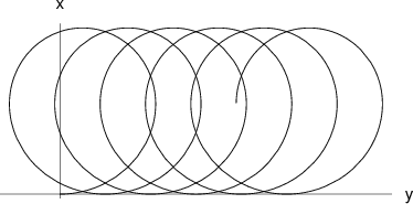
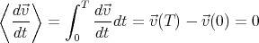
- The drift velocity is the particle’s velocity vector
 averaged over a
complete cycle in the periodic trajectory:
averaged over a
complete cycle in the periodic trajectory:  D =
D =  ∫
0T
∫
0T  dt = ⟨
 ⟩. In a
homogeneous magnetic field
⟩. In a
homogeneous magnetic field  0, the average of the velocity
  0
is ⟨
0
is ⟨ 0⟩ = 0. If the magnetic field is perturbed with a small
 ′, the change
  ′(t) =
  (t) -
(t) - 0(t) in the velocity will also be
small. Note that this is true only because in this problem
0(t) in the velocity will also be
small. Note that this is true only because in this problem  (t) is
periodic.
(t) is
periodic.
The motion of the particle is governed by the equation
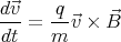
Let us take the average of both sides of this equation over a complete cycle:
Thus,
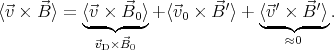
For calculating ⟨
 0 ×
0 × ′⟩, we again approximate the actual trajectory
with the non-perturbed one:
′⟩, we again approximate the actual trajectory
with the non-perturbed one:

= R(cos ωt, sin ωt, 0)  0 =
0 = 
= v(- sin ωt, cos ωt, 0)
Integrating these expressions over (0,T) we get ⟨(  0 ×
0 × ′)x
′)x= (v0)ykx = kRv cos 2ωt (  0 ×
0 × ′)y
′)y= -(v0)xkx = kRv sin ωt cos ωt  0 ×
0 × ′⟩ = Rv0 k
 ∕2.
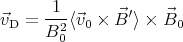
Defining
∕2.
Defining  = k
= k , the drift velocity is
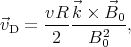
where R = mv∕qB0.