Let ρ denote the charge density, and ω the angular velocity.

Let us divide the cylinder into thin cylindrical shells. A shell of radius r will have a surface current density K = ρωrdr. To find the magnetic field of such a shell, imagine that we bend it into a torus with perimeter p. In the limit p →∞ the torus is an infinitely long cylindrical shell, and we do not need to distinguish between its inner and outer perimeters. Using Ampère’s law and integrating along the “centre ring” of the torus we find that B = μ₀K inside the torus. This also holds for a straight cylindrical shell. Outside B = 0.

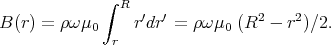
Summing up the contributions of the shells we find that the magnetic field at distance r from the axis of the cylinder is

∫ R ′ ′ 2 2 B (r) = ρ ωμ0 rdr = ρω μ0 (R - r )∕2. r

The potential created by a bounded charge distribution at point

is

∫ ⃗ --1-- |-ρ(⃗r)|- 3 V(R ) = 4π ε0 |⃗ | d ⃗r. |R - ⃗r|

For simplicity let us consider -1--
4πε0 ≡ 1 below.

Let the components of vectors and be denoted

⃗ R = (X, Y,Z ) = (X1,X2, X3 )

⃗r = (x,y,z) = (x ,x ,x ), 1 2 3

and let F() = 1∕ || ||
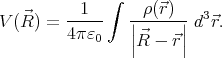
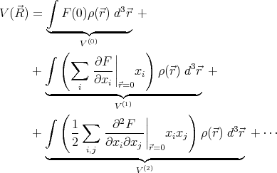
|⃗R - ⃗r| . Now let us expand F() in Taylor series, and write the potential as

∫ ⃗ 3 V (R ) = F (0)ρ(⃗r) d ⃗r + ◟------◝◜-----◞ ( V (0) ) ∫ ∑ ∂F || + ---|| xi ρ(⃗r) d3⃗r + i ∂xi ⃗r=0 ◟------------◝◜(1)-----------◞ ∫ ( V | ) 1 ∑ ∂2F | 3 + -- -------|| xixj ρ(⃗r) d ⃗r + ⋅⋅⋅ ----2-i,j--∂xi∂xj ⃗r=0-------------- ◟ ◝(◜2) ◞ V

(1)

Here V ⁽⁰⁾ is the monopole term in the expansion of the potential, V ⁽¹⁾ is the dipole term, V ⁽²⁾ the quadrupole, etc.

Let us define A, A_i, A_ij, … in the following way:

	= F(0)
	= ₌₀
	= ₌₀
…

Now the terms of the potential’s expansion can be written as

V ⁽⁰⁾	= A∫ ρ() d³
V ⁽¹⁾	= ∑ _iA_i ∫ x_iρ() d³
V ⁽²⁾	= ∑ _i,j ∫ x_ix_jρ() d³
…

Note that the coefficients A, A_i, … only depend on ⃗
R , but not . If we carried out the tedious calculations, for the first few A-constants we would get A = 1, A_i = X_i, A_ij = 3X_iX_j - δ_ijR², where δ_ij is the Kronecker delta.

The monopole term in the potential is just proportional to the total charge ∫ ρ() d³ = Q, and does not depend on , hence it does not depend on the choice of origin of our coordinate system. What happens to the dipole term if the origin of the coordinate system is changed, or, equivalently, the charges are shifted by a vector = (a₁,a₂,a₃)?

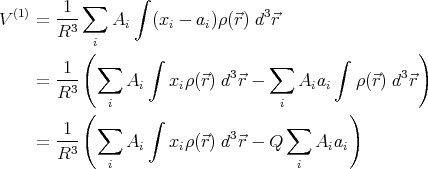∫ (1) 1--∑ 3 V = R3 Ai (xi - ai)ρ(⃗r) d ⃗r (i ) 1 ∑ ∫ ∑ ∫ = -3- Ai xiρ(⃗r) d3⃗r - Aiai ρ(⃗r) d3⃗r R i i ( ∑ ∫ ∑ ) = 1-- A x ρ(⃗r) d3⃗r - Q A a R3 i i i i i i

Note that if the total charge (and the monopole term in the potential) is 0, then V ⁽¹⁾ does not change when the charges are shifted.

Now suppose that V ⁽¹⁾ = 0 for any , and thus ∫ x_iρ() d³ = 0 for each i. When the charges are shifted, V ⁽²⁾ will be

∑ ∫ V (2) = -1- Aij- (x - a )(x - a )ρ(⃗r) d3⃗r R5 2 i i j j i,j ( ) 1 ∑ Aij ∫ 3 1 ∑ ∑ ∫ 3 = --5 ---- xixjρ(⃗r) d ⃗r ---5 Aijaj xiρ(⃗r) d ⃗r+ R i,j 2 R i j 1 ∑ Aijaiaj ∫ + --5 ------- ρ(⃗r) d3⃗r R i,j 2

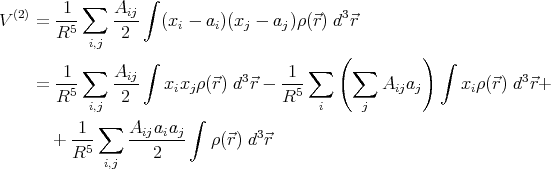Here we used the fact that A_ij = A_ji to simplify the result. Note again that if ∫ ρ() d³ = 0 and ∫ x_iρ() d³ = 0, then V ⁽²⁾ does not change when shifting the charges.

It can be shown in a similar way that any V ⁽ⁿ⁾ will be independent of the choice of origin of the coordinate system if V ⁽ⁱ⁾ = 0 for all i < n and all ⃗
R .

Adding one more “step” to the infinite ladder will not change it. Let R_L denote the resistance of the ladder.

Figure 1:

Adding one more step to the ladder (represented by R_L) does not change its resistance. Thus the resistance between points A and B is R_L as well.

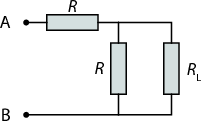
The configuration of figure 1 must have resistance R_L too:

( ) 1 1 - 1 RL = R + --+ --- R RL

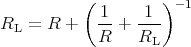
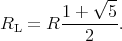
The positive solution of this equation is

√ -- 1 + 5 RL = R ---2---.

If we let a current I flow into point A, the current though the resistor between A and B will be I∕4 (because of the symmetrical arrangement of the resistors, see fig. 2). Therefore the voltage drop across resistor AB is U₁ = RI∕4.

Figure 2:

When current I is flowing into point A, the current through resistor AB is I∕4.

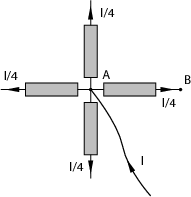
Similarly, if a current I is flowing out from point B, the voltage drop across resistor AB is U₂ = RI∕4.

According to the principle of superposition, when we have both a current I flowing into point A and a current I flowing out from point B, the voltage drop across AB will be U_total = U₁ + U₂ = 2 ×RI∕4. The resistance between points A and B is U_total∕I = R∕2.

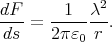
Let us calculate the force between the wires in both cases:

Using Gauß’s law we find the electric field at distance r from a wire E = 1∕2πε₀ λ∕r (λ is the linear charge density). The force on unit length ds of the other wire is $dF 1 λ2 --- = -------. ds 2πε0 r$
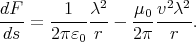
The moving wires have a current I = vλ. It is easy to find the magnetic field using Ampère’s law (integrate along circular loops around the wire): B = μ₀∕2π vλ∕r. The force due to the magnetic interaction is attractive, so the total force is $dF- -1---λ2- μ0-v2λ2- ds = 2πε r - 2π r . 0$

The results in points (a) and (b) are not identical. However, the two presented situations are exactly the same setup, viewed from different reference frames.

This is a good illustration of Maxwell’s equations not being invariant to the classical Galilei–transformation (x′ = x - vt; t′ = t). If we take into account the change in charge density due to the relativistic Lorentz–contraction, λ′ = λ∕ ∘ ---------
1 - v2∕c2 , it is easy to show that the force is the same in both reference frames. (Use the relation ε₀μ₀ = 1∕c².)