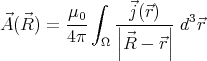
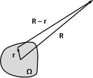
(See fig. 1 for notations.) The first term of the multipole expansion is
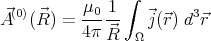
Therefore it is sufficient to prove that the volume integral of the current
density over Ω is 0. For this, let us calculate the divergence of  x, where x is
a position coordinate!
x, where x is
a position coordinate!
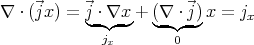
We know that for any current and charge distribution ∇⋅ j +  ρ = 0,
therefore in the stationary case ∇⋅j = -
ρ = 0,
therefore in the stationary case ∇⋅j = - ρ = 0. So the x component of the
volume integral of
ρ = 0. So the x component of the
volume integral of  can be written as

Using the Gauß–Ostrogradksi theorem, the volume integral on Ω can be
converted into a surface integral on over the boundary ∂Ω. But there are no
currents outside the domain Ω, so the volume integral can be extended into
a slightly bigger region (one the boundary of which  = 0), therefore the
surface integral is 0.
= 0), therefore the
surface integral is 0.
The same reasoning can be applied to prove that the projection of the volume integral along any any axis is 0.
 is 0. Suppose that the normal component weren’t
zero: in this case the surface integral of
is 0. Suppose that the normal component weren’t
zero: in this case the surface integral of  over a “pillbox” surface around the
surface of the superconductor would be non-zero, which contradicts the
Maxwell-equation ∇⋅
over a “pillbox” surface around the
surface of the superconductor would be non-zero, which contradicts the
Maxwell-equation ∇⋅ = 0.
= 0. 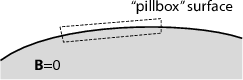
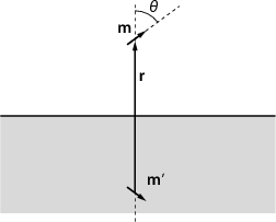
Now let us calculate the force acting on a small magnet above a superconducting plane! We can use the method of images: The normal component of the magnetic field, B⊥, must be zero just above the surface. This could be achieved by removing the superconducting plane and inserting another small magnet, one that is exactly the mirror image of the original magnet with respect to the plane (see fig. 2). The magnetic field is determined at all points in space if the boundary conditions are specified. Therefore the magnetic field in the “upper” half-space will be the same in the presence of the superconductor as without the superconductor, but with the mirror magnet. The force on the magnet will be just the same as the force exerted by the mirror-magnet.
The vector potential of a magnetic monopole  is
is
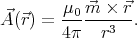
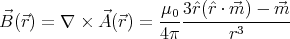
 is the position vector relative to the magnet. By taking the curl we find
the magnetic field:
is the position vector relative to the magnet. By taking the curl we find
the magnetic field:
The energy of a magnetic dipole  in a field
  is W = -
 ⋅
⋅ , and the
force acting on it is F = -∇W.
, and the
force acting on it is F = -∇W.
Let the dipole moment of the magnet be  , the dipole moment of the mirror
magnet be
, the dipole moment of the mirror
magnet be  ′. The energy associated with them is
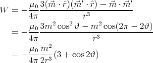 |
The force acting on the magnet is
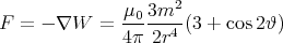
The magnet will adopt an orientation that minimizes its energy, i.e. maximizes cos 2ϑ: ϑ = 0 or ϑ = π. The magnet’s axis will be perpendicular to the superconducting surface.
It is a legitimate question to ask: how do we come to the conclusion that the mirror charge distribution must be a linear dipole? We saw on the lecture that a dielectric of any shape can be imagined as two superposed homogeneous charge distributions, one positive and the other negative. When there is no external field, they cancel out, but when a field is applied, they separate by a very small distance.
If we are concerned only about electrostatics, a dielectric of εr →∞ can be considered equivalent to a conductor. This may suggest that taking two oppositely charged solid cylinders, slightly separated in a direction perpendicular to their axis, will give the correct mirror charge distribution. According to Gauß’ law, outside the cylinder the field of this configuration is the same as the field of a linear dipole.
The final result is:


where ϑ is the angle measured from the direction of  along the cylinder’s
perimeter.
along the cylinder’s
perimeter.